
Application of signal processing techniques to the detection of tip vortex cavitation noise in marine propeller*
2013-06-01 12:29LEEJeungHoonHANJaeMoonPARKHyungGilSEOJongSoo
水动力学研究与进展 B辑 2013年3期
LEE Jeung-Hoon, HAN Jae-Moon, PARK Hyung-Gil, SEO Jong-Soo
Samsung Ship Model Basin (SSMB), Marine Research Institute, Samsung Heavy Industries, Science Town, Daejeon 305-380, Korea, E-mail: jhope.lee@samsung.com
Application of signal processing techniques to the detection of tip vortex cavitation noise in marine propeller*
LEE Jeung-Hoon, HAN Jae-Moon, PARK Hyung-Gil, SEO Jong-Soo
Samsung Ship Model Basin (SSMB), Marine Research Institute, Samsung Heavy Industries, Science Town, Daejeon 305-380, Korea, E-mail: jhope.lee@samsung.com
(Received July 27, 2012, Revised March 15, 2013)
The tip vortex cavitation and its relevant noise has been the subject of extensive researches up to now. In most cases of experimental approaches, the accurate and objective decision of cavitation inception is primary, which is the main topic of this paper. Although the conventional power spectrum is normally adopted as a signal processing tool for the analysis of cavitation noise, a faithful exploration cannot be made especially for the cavitation inception. Alternatively, the periodic occurrence of bursting noise induced from tip vortex cavitation gives a diagnostic proof that the repeating frequency of the bursting contents can be exploited as an indication of the inception. This study, hence, employed the Short-Time Fourier Transform (STFT) analysis and the Detection of Envelope Modulation On Noise (DEMON) spectrum analysis, both which are appropriate for finding such a repeating frequency. Through the acoustical measurement in a water tunnel, the two signal processing techniques show a satisfactory result in detecting the inception of tip vortex cavitation.
tip vortex cavitation, inception, Short-Time Fourier Transform (STFT), Detection of Envelope Modulation On Noise (DEMON)
Introduction
The tip vortex cavitation is treated as the main source of noise contributor in marine propeller. It has been already become of interest to the marine engineers not only because of its first appearance among the other types of cavitations, but also because of the influential sound pressure level dwelling in a broadband[1-3]. More specifically, the onset of tip vortex cavitation, a situation when it firstly takes place, lies in a primary concern for the commercial- or the militarypurpose. As the regulation for the environmental impacts from commercial ships becomes stringent, the propeller cavitation noise needs to be predicted beforehand. In this case, model-scale measurement is extrapolated with an aid of priory known cavity-inception characteristic[4,5]. Furthermore, the cavitation inception dominates an underwater surveillance of naval-ship by limiting its operational range. In either case, the accurate determination of cavitation inception is a prerequisite.
Conventional power spectrum analysis for an acoustical measurement is normally employed for an inception criterion. An increase within a certain frequency band of the power spectrum in a comparison with a non-cavitating condition can be a sign of the cavitation inception. This approach can be practical if the acoustical signature is pre-identified for various cavity patterns, which is not in the majority of cases. In addition, when the other cavitation noise sources exist except the tip vortex, it can be ambiguous to detect the tip vortex cavitation.
Note that tip vortex cavitation of propeller and its bursting noise is repeated in a periodic manner, alternatively, thus finding the repeating frequency of bursting from the relevant acoustic signal can be considered as a basic strategy to recognize the cavitation inception. This naturally leads to employ the Short-Time Fourier Transform (STFT) analysis[6]and the Detection of Envelope Modulation On Noise (DEMON) spectrum analysis[7], both which are popular algorithms in the machine diagnostic field. The former is to decompose the signal into both time and the frequencydomains, and consequently to observe (or count) the spectral variation with time. The latter is to analyze the spectrum of the envelope for the original signal possessing only the low frequency contents, i.e., the repeating frequencies.
This paper will concentrate on their applicability to the detection of cavitation inception. Section 1 covers the noise characteristics at an initial stage of cavitation as well as the brief introduction to the two techniques. Analysis with the actual measurement will be dealt in Section 2. The pros and cons for those techniques will also be given. Finally, this paper closes with conclusions in Section 3.

Fig.1 Axial velocity distribution in the plane of propeller for a typical single-screw merchant ship

Fig.2 Velocity diagram of blade section at certain propeller radius r
1. Basic theory and techniques for cavitation detection
1.1 General noise characteristics of cavitation
When the pressure in a liquid is reduced below a certain critical value, i.e., the vapor pressure, the nuclei existing in the liquid begins to grow. After the pressure has been re-increased above the critical value, the vapor bubble formed around the nuclei begins to collapse implosively and finally disappears. Such a violent process of cavity collapse takes place in very short time duration of several micro-seconds and results in a radiation of bursting or impulsive noise[8]. This phenomenon is known as cavitation and treated as the most prevalent noise source in marine propeller.

Fig.3 Schematic representation of repeated bursting noise. The series of damped bursts are assumed as identical and perfectly uniformly spaced by T. It is further assumed that the each burst has single frequency of oscillationf0much higher than 1/T
As the propeller blade rotates behind the ship, each section of the blade experiences a fluctuation of inflow velocity resulting in periodic occurrences of cavitation. Figure 1 shows an axial inflow velocity distribution in the plane of propeller for a typical single-screw merchant ship. Lower velocity region caused by the hull shadow is visible around the top of the propeller disk. Then the velocity diagram of blade section at a certain propeller radius r can be represented by Fig.2. The angle of attack αbecomes large for a smaller magnitude of axial velocity, and subsequently the liquid on the blade surface is prone to cavitate. Whenever each blade passes through such a lower velocity region in Fig.1, the occurrences of cavitation will be repeated periodically. Hence, the noise radiation pattern from the propeller cavitation can be schematically represented by periodic repetitions of bursting noise as shown in Fig.3. Bursting noise itself contains a high-frequency component ranging several tens of kilo-hertz, but its repeating frequency corresponding to blade passing frequency is relatively low.
Conventional power spectrum analysis can be firstly considered for the detection of cavitation inception. However, as was mentioned in Introduction, it requires extensive experimental studies to correlate various cavity patterns with its noise signature, which is far beyond our research scope. Furthermore, when the other noise sources such as cavitation on the strut, rudder and etc. exist, the spectral analysis cannot be practical in finding the propeller cavitation. In the signal processing field, the diagnostic information is often contained in the repeating frequency rather than in their frequency content of bursting noise[9]. Thus, an alternative way for detection would be expected to find the repeating frequency, and to decide whether itcoincides with the blade passing frequency or not.
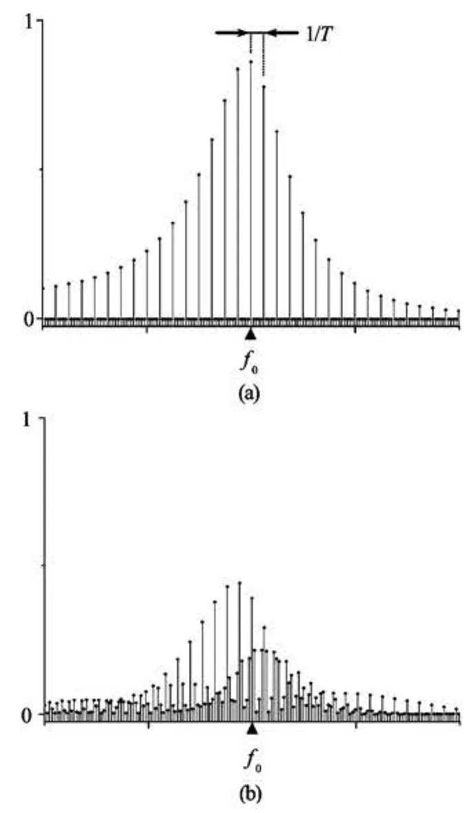
Fig.4 Power spectrum plots for the assumed signals, (a)when the bursts have identical and perfectly uniform time-spacing like the signal in Fig.3, and (b)when there are slight variations between their time-spacing. For clarity, the frequency resolution for the former case is given by 1 / (5T), since the whole five series of bursts shown in Fig.3 were used for the estimation of power spectrum. In the latter spectrum, the same frequency resolution(=1/ (Nd t))was maintained by adding some zeros in the tail of the signal, whereNis the number of data points used in the computation of the former spectrum, anddtthe sampling time
Let us assume a series of bursts possessing perfectly uniform spacing byT as shown again in Fig.3. It is further assumed that each burst has only one oscillation frequency f0much higher than1/T(the repeating frequency). Its resultant power spectrum as shown in Fig.4(a) will be another train of impulses with frequency spacing1/T, and with the largest values at the oscillation frequency f0of the burst. The repeating frequency, in principle, could be found by measuring the frequency spacing of the harmonic series in the vicinity of the fundamental oscillation frequency. However, actual measurements have slight variations between the bursts and also in their timespacing, so that the impulses in the spectrum tend to spread over the sideband, and merge with other one as represented in Fig.4(b). Measuring the repeating frequency using a conventional spectrum is eventually impractical.


where w( t-τ)is a window function moving along the record. Normally, the Hanning tapering[6]is employed as a window function.
At this point, the STFT analysis should be mentioned that a high resolution cannot be obtained simultaneously in both the time- and the frequency-domains. If the width of the window for a segmented record isTB, then corresponding frequency resolution is given by 1/TB, which must be decided based upon the specific characteristic of the data being analyzed. Although a shorter data window (with smallerTB) would give a better time resolution in the time-frequency diagram, the resolution in the frequency axis should be necessarily compromised. That is, the two requirements of a short data window and a narrow frequency resolution are incompatible. In spite of such a restriction, STFT is still useful for tracking the changes in frequency with time.
Other approach for the time-frequency analysis is to consider the Wigner-Ville distribution[6]or wavelet transform[10]. Due to a better resolution than STFT, they were successfully applied in several applications such as local fault detection in a structure. However these alternatives provide no significant benefit over the STFT analysis especially for treating the cavitation noise.
1.3 DEMON spectrum analysis
By referring Fig.3 again, one needs to note that a carrier or a high-frequency component of bursting noise is amplitude-modulated by a repeating frequency, which is much lower than the carrier component. If an envelope of original signal overlaid in Fig.3 is formed by amplitude demodulation, then spectral analysis of the envelope signal, instead of the original one, will reveal a repetition frequency directly. This idea, referred as DEMON spectrum (or frequently referredas envelope spectrum), can be extremely useful when the cavitation noise is modulated by a constant repeating frequency.
The procedures to compute DEMON spectrum are detailed in the following. At first, the measured raw signal in time domain needs to be band-pass filtered around the relevant frequency ranges of propeller cavitation. This eliminates not only low-frequency components that are common in rotating machinery including shaft misalignment, unbalance, but also other noises that are not directly related with propeller cavitation. Practically, the filtering is the most important step because the quality of DEMON spectrum highly depends on detecting and enhancing an impulsiveness of the signal to be analyzed[11]. In spite that there is still a debate on how to choose the most suitable band for demodulation, a practical way in the present is to examine the power spectrum for various operating conditions. In detail, an increase within a certain frequency band in comparison with a cavitation-free situation can indicate the presence of cavitation, and consequently provide an appropriate band for filtration as well.
Next step is to form an analytic signal xa( t)by using the filtered signalxf(t),
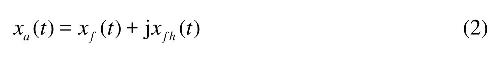
where xfh(t )is the Hilbert transformation[6]of xf(t) defined by the following
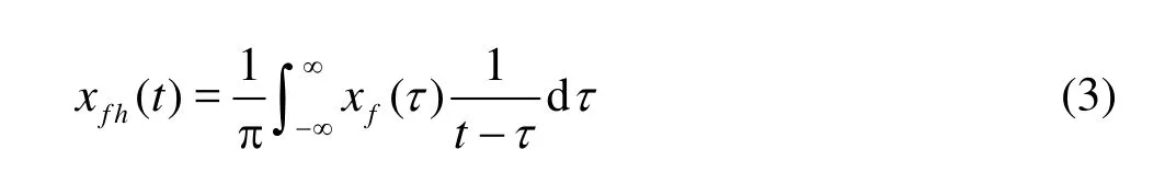

where the symbol ⊗denotes a convolution integral.
Then the amplitude of analytic signal gives the envelopexe( t )as follows

Finally conventional spectral analysis for the resulting envelope is made to extract the repeating frequency component.
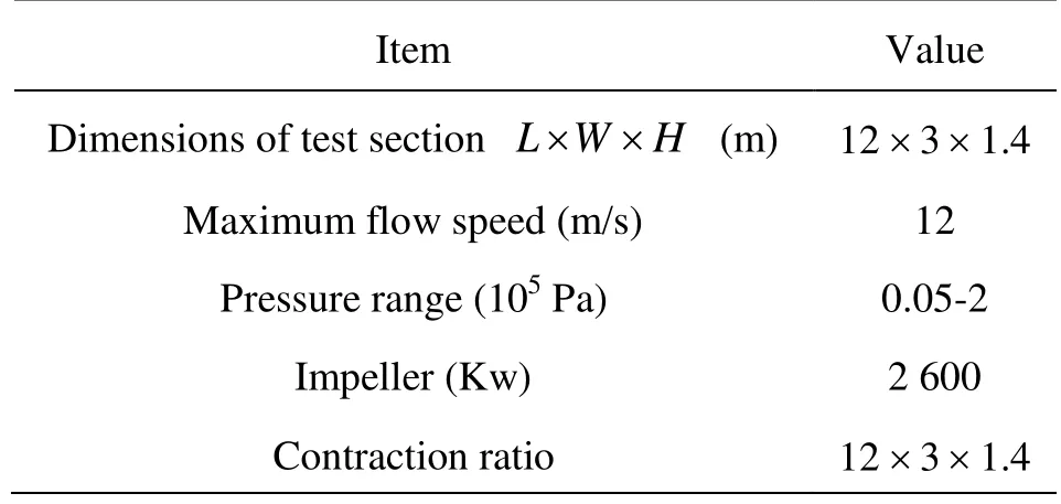
Table 1 Principal particulars of test section
2. Application of the detection techniques to experimental measurements
2.1 Test procedure and result of noise measurement
Two techniques of signal processing for the detection of tip vortex cavitation noise were discussed in the previous section. To examine their applicability, acoustical measurements for a model ship equipped with a six-blades propeller were performed in the water tunnel of the Samsung Ship Model Basin (SSMB). The principal particulars of the tunnel are summarized in Table 1. The test section of 3.0 m width, 1.4 m height and 12.0 m length is able to accommodate the complete ship model. Inside the model ship, a water tight dynamometer was installed for the measurement of thrust, torque and RPM of the model propeller. Wooden plates are placed between the tunnel wall and the model ship at the height corresponding to the scaled design draught to suppress free water surface. Figure 5 shows the complete model ship installed in the water tunnel.

Fig.5 Complete model ship mounted in the water cavitation tunnel of SSMB
The miniature hydrophone (model: B&K 8103) was also flush-mounted on the hull surface just above the propeller. The signal from the hydrophone passed through the signal conditioner (model: B&K 2690),and logged into the PC-based measurement system with a sampling frequency of 256 kHz.
One may argue with the problem of a near-field noise measurement[13], because the distance between the sensor and the acoustic center of cavitation is too close by less than 0.1 m. The low-frequency data can be definitely suffered from a fluctuation provoked by near field measurement. Unfortunately the tunnel has no suitable place for the sensor which can meet the requirement of far-field measurement. Alternatively, a long-time signal of 120 s was recorded for each measurement to give an enough average on spectrum estimates. Besides, three additional hydrophones were installed around the stern hull surface to observe whether there exists large differences between the readings. This issue will be discussed further with the measured data.
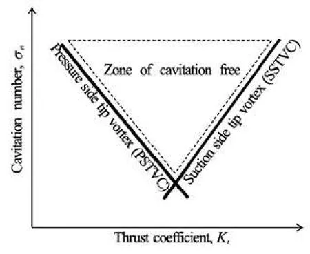
Fig.6 Schematic diagram of tip vortex caivtation inception

Fig.7 Cavitation inception diagram for the employed propeller and acoustic noise measurement points
The propeller is tested at a prescribed set of two non-dimensional numbers: thrust coefficient Ktand cavitation number σn
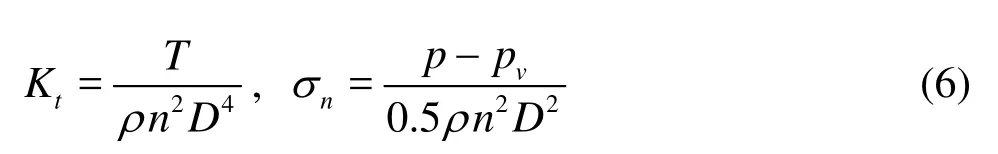
where T denotes the thrust force of propeller,ρthe water density,nthe rate of revolution of propeller (rps),D the diameter of propeller,p the pressure in the tunnel, and pvthe saturated vapor pressure depending on temperature. To reach the propulsion point, the flow speed in the tunnel is firstly controlled. Then the propeller rps is adjusted to the value giving the desired thrust coefficient on the basis of the thrustidentity[14,15]. After achievingthethrustidentity,the tunnel pressure is controlled to match a prescribed cavitation number.

Fig.8 Definition of blade angle

Fig.9 Images taken by high-speed camera for the test condition number 1 with the time interval between the images of 0.56 ms
A typical inception diagram of tip vortex cavitation is represented on a plot of thrust coefficient Ktand cavitation number σnas schematically shown in Fig.6. At small values of thrust coefficient yielding anegative angle of attack α, the tip vortex cavitation is prone to occur at the pressure-side of the blade. For an increased thrust coefficient but still α<0, an incipient cavitation number of Pressure Side Tip Vortex Cavitation (PSTVC) will be lower than the former case. As the thrust coefficient is further increased to give a positive angle of attack, the PSTVC disappears and tip vortex cavitation at suction-side (SSTVC) becomes to emerge. On the contrary to the PSTVC, the SSTVC at a high loading will be detected at a higher cavitation number than the one at a lower loading. Therefore, a typical inception diagram for tip vortex cavitation exhibits a V-shape curve, the above of which designates a region of cavitation free.

Table 2 Summary of noise measurement condition and blade indices of incepted tip vortex
Due to tip-loaded characteristic of the employed propeller, yet, the pressure-side tip vortex caviation could not be generated, consequently only the suctionside tip vortex cavitation was investigated. Further tip vortex cavitation, especially in model propeller, does not occur simultaneously at all blades due to a geometrical tolerance, instead one or two blades among the other reveal an early tip vortex. In our case, one blade among the six begins to exhibit a cavitation, which is not regarded as an inception in a normal practice of model test.
Once a cavitation occurs, however, noise level would exhibit a significant increase irrespective of the number of cavity-incepted blades. Considering that this work employs the acoustic data as an inception criterion, thus, the cavitation occurrence at one blade only will be considered as the condition of inception. Based on such criterion, the inception diagram for the employed propeller was prepared through a visual inspection, as shown in Fig.7. All the tip vortex were observed at the blade angular position between –10oto 10o, the definition of which is depicted in Fig.8. For reference a series of images taken by high speed camera is shown in Fig.9.
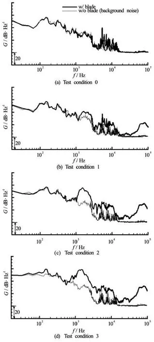
Fig.10 Power spectral densities for noise measurement and comparison with the background noise. Processing parameters: Hanning window, 1 000 times ensemble average, 75% overlapping, narrow bandwidth frequency resolution of 16 Hz
Acoustic noise measurements were conducted by varying the cavitation number σnfrom 9.013 to 7.041 whilst keeping the thrust coefficient as a constant, i.e., Kt=0.205. Corresponding points are marked with “•”symbol in Fig.7. Table 2 summarizes noise measurement conditions aswe ll as indice s of the cavity-inceptedblades.Figure10representsmeasuredsignalforeach condition, where the power spectral densities were estimated by using the Hanning window and ensemble average of 1 000 times with over-lapping of 75%, and observed with narrow frequency resolution of 16 Hz[6]. For a validation of measured signal, background noise measurements were also performed under the configuration of dummy hub, i.e., without the propeller blades. At the non-cavitating condition in Fig.10(a), background noise seems to have significant influence for the whole frequency range. Shaft rotation together with water flow in the tunnel would have affected on the low frequency range below 100 Hz. Also the noise from a motor-driving inverter influences to several harmonic tones between 4 kHz and 15 kHz, which needs to be excluded in later analysis. Basically the non-cavitating noise originated from a blade loading or a thickness is regarded as insignificant for the employed propeller.
On the contrary, when there exists cavitation, the spectrums given in Figs.10(b)-10(d) show a distinct increase in the frequency range of 1 kHz-3 kHz and 40 kHz-100 kHz. Measurements with blades for those frequency ranges are approximately 10 dB larger than the background, which demonstrates a validity of measured data in the cavitating conditions. To make sure an effect of near-field instability, furthermore, measurement at additional locations nearby a central hydrophone were compared together, and found to be fluctuating only below 100 Hz.

Fig.11 Collection of power spectral densities for measurements with blade
For convenience, measurement cases with blade are collected in Fig.11. As the cavitation number decreases, that is, as the tip vortex cavitation develops, sound pressure level increases within two frequency ranges where were mentioned above. Firstly, with the enlargement of sound pressure level between 1 kHz to 3 kHz, the frequency of maximum in that range fmaxshifts to the lower from 1.8 kHz to 1.4 kHz. If we assume the tip vortex as an equivalent single macrobubble, the shifting phenomenon can be explained by the resonance frequency of gas bubble in liquid which was firstly proposed by Minnaert[3]

In the above,p denotes the pressure,a0the volume of equivalent cavitating bubble,γ(=1.4)the specific heat ratio of air andρthe density of water. Although it is not possible to estimatea0precisely, visual inspection could yield its rough estimate around several millimeters. Furthermore, average size was not increased significantly during the depressurization. Afterward,fmaxdwells between 1.1 kHz and 1.5 kHz, which is a quite similar frequency range showing a shifting phenomenon. Therefore we can consider the noise in the frequency band 1 kHz-3 kHz would be related with volumetric resonance of tip vortex cavitation.
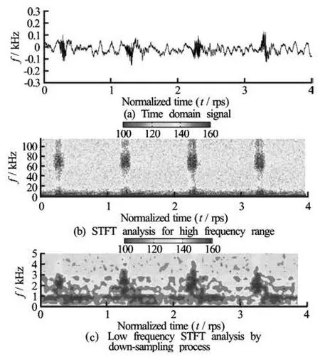
Fig.12 Time signal and STFT analysis for the four periods of propeller revolution at the test condition number 1. Unit of contour level is in dB with the dB reference value of 1 µPa)
On the other hand, it is somewhat ambiguous for noise increment between 40 kHz and 100 kHz. Several individual micrometer-sized bubbles constituting the single macro bubble and their resonances are suspected to be the origin of noise increment in high frequency ranges. Because noise characteristics in a high-frequency range above 20 kHz was scarcely treated in the literatures, however, such a noise increment can be argued by development of traveling bubble in the tunnel during the depressurization or by several sources rather than the tip vortex cavitation. As has been seen above, although an increase of sound pressure level can be qualitatively noticed with the decrease of cavitation number, typical spectral analysisin Fig.11 does not provide an apparent clue for the cavitation inception.
2.2 Results of STFT analysis
For the condition where the tip vortex cavitation was incepted at one blade only, Fig.12(a) depicts measured acoustic signal in time domain for the period of four shaft revolutions, and Fig.12(b) the corresponding STFT analysis. Only single impact-like event ranging between 40kHz and 100kHz can be observed for each revolution. Also it is periodically repeated with an interval of shaft rate providing an evidence of cavitation inception. Meanwhile, Fig.12(c) depicts the STFT result for low-frequency range, obtained with the down-sampling (decimation) method[6].

Fig.13 STFT analysis for each test condition, The four periods of propeller revolution were analyzed
Distinctness in contour color is obscure due to other noise sources. It is hard to disclose that the frequency component between 1 kHz and 3 kHz where another frequency range of tip vortex is repeated by the shaft rate. When the contribution of other noise sources beyond the tip vortex is not negligible, the STFT analysis can be frustrated. This means the timefrequency diagram is vulnerable to an additional source coexisting in the interested frequency band. Further example of unsatisfactory result can be found at Fig.12(b) of authors’ paper[5], in which STFT analysis was applied to measurement at a full ship. In that case, cavitation detection based on STFT was disturbed by the combustion noise of main engine. Thus the authors emphasize that STFT is not the sole analysis tool for cavitation detection.
However, provided that signal-to-noise ratio is high enough, STFT returns acceptable results as shown in Fig.13. By referring to Table 2, we can see that the number of impact events within one shaft revolution is identical to the one of cavity-incepted blades. Based on the above analysis, STFT analysis can be considered as an indication tool for cavitation inception in spite of its weakness to a noise.

Fig.14 Example of the DEMON spectrum estimation at the test condition number 1
2.3 Results of DEMON analysis
Figure 14 facilitates understating the principles of DEMON spectrum. Figure 14(a) shows again a raw time history at the condition of cavitation inception at one blade only. High-frequency oscillation per one shaft revolution, i.e., the bursting noise from the cavitation is not clear because the concatenated low frequency ringing is in a quite similar amplitude with high-frequency component. As was explained in Section 1.3, the signal needs to be band-pass filtered to enhance its impulsiveness. The appropriate frequency for the filter was chosen as 40 kHz-100 kHz based on the power spectral densities in Fig.11. The black line in Fig.14(b) represents the filtered signal exhibiting a high signal-to-noise ratio. The overlaid thick line is the envelope of filtered signal, which is processed by the FFT algorithm to give the DEMON spectrum in Fig.14(c). The white tick marker on the top of each DEMON spectra denotes the frequencies of propeller rps and its harmonics. Especially, every sixth ticks were spotted with a thick marker to represent blade frequency components. We can see an emergence of shaft frequency and its harmonic compone-nts at the DEMON spectrum. As was stated earlier, the key idea of DEMON is to analyze the repeating frequency of impact-like signal, not the frequency contents of the original signal itself. We have already seen in Fig.14(a) that the repeating time interval of impact-like signal is an inverse of the propeller rps. Hence, the modulus of DEMON spectrum has the highest value at the frequency component of propeller rps, the so-called shaft frequency modulation.

Fig.15 DEMON spectrum when the band-pass filter frequency is chosen between 1 kHz and 3 kHz
If the frequency range of band-pass filter is chosen as 1 kHz-3 kHz, the corresponding DEMON spectrum shown in Fig.15 is still dominated by the shaft frequency. These are comparable to the former STFT analysis in Fig.12(c), whose results were rather cumbersome to detect the cavitation inception in that frequency range. Thus, the DEMON analysis is regard as better than the STFT technique in an aspect of robustness to external noise.

Fig.16 DEMON spectrum for each test condition, Band-pass filter frequency: 40 kHz-100 kHz, Unit of contour level is modulus of DEMON spectrum
DEMON spectrums for the other test cases are represented in Fig.16. At non-cavitating condition depicted in Fig.16(a), no diagnostic frequency component is available, which implies no cavity on the propeller blade. For the inception condition at four blades, the corresponding DEMON analysis in Fig.16(c) exhibits 2xshaft frequency modulation. By referring to peller rps) sec, resulting at the2xshaft frequency modulation in the DEMON spectra. When the tip vortex cavitation is incepted at all blades, we can definitely find the blade frequency modulation as shown in Fig.16(d).
In short, once the cavity occurs on a propeller blade, the corresponding DEMON spectra certainly shows distinctive values at a shaft frequency or its harmonics. For a further developed cavitation, blade frequency rather than shaft one becomes to emerge. Thus the appearance of shaft- or blade-frequency related components in DEMON provides a clear evidence of cavitation inception, which fascinates over classical spectral analysis technique. Fig.13(c) and Table 2 as well, the indices of incepted four blade are not in a sequential order. The cavity is missed at the blade indices of A and D. This means the two groups of impact-like signals at blade indices B, C and E, F is repeated by the interval of 1/(2×pro-
3. Concluding remarks
It is the purpose to detect tip vortex cavitation in marine propeller based on acoustical measurements. Basic strategy is to extract the repeating frequency of cavitation for a measured record, and to decide whether it coincides with the shaft- or blade-passing frequency. Owing to its limitation in the resolution capability, typical analysis by power spectrum is impractical to employ. Instead, two signal processing techniques which are popular in a machine diagnostic field have been considered for the alternatives. One is STFT analysis decomposing the signal into both time and frequency domain, and observing the variation in frequency with time. The other is DEMON spectra analyzing the envelope of signal that is formed by an amplitude demodulation.
We could observe that these two techniques have been successfully employed for identifying the tip vortex caivtation generated in a water tunnel. In a case when the time-frequency diagram of STFT is disturbed by other noise sources, DEMON spectra complementary shows an evidence of cavitation inception. From the analysis discussed so far, DEMON spectrum together with STFT analysis can be adhered as useful tools for the decision of cavitation inception, the example of which can be found in the authors’ another paper[5]as well.
[1] RICHARD P. Underwater acoustics[M]. New York, USA: John Wiley and Sons, 2010.
[2] CARLTON J. Marine propellers and propulsion[M]. 2nd Edition, USA, Massachusetts: Butterworth- Heinemann, 2007.
[3] MEDWIN H. Sound in the sea: From ocean acoustics to acoustical oceanography[M]. Cambridge, UK: Cambridge University Press, 2005.
[4] SHEN Y. T., GOWING S. and JESSUP S. Tip vortex cavitation inception scaling for high Reynolds number applications[J]. Journal of Fluids Engineering, 2009, 131(7): 071301.
[5] LEE Jeung- Hoon, JUNG Jae-Kwon and LEE Kyung-Jun et al. Experimental estimation of a scaling exponent for tip vortex cavitation via its inception test in full- and model ship[J]. Journal of Hydrodynamics, 2012, 24(5): 658-667.
[6] BENDAT J. S., PIERSOL A. C. Random data: Analysis and measurement procedures[M]. 4th Edition, New York, USA: John Wiley and Sons, 2010.
[7] RANDALL R. B. Vibration-based condition monitoring[M]. New York, USA: John Wiley and Sons, 2011.
[8] FRANC J., MICHEL J. Fundamentals of cavitation: Fluid mechanics and its applications[M]. Dordrecht, The Netherlands: Kluwer Academic Publishers, 2010.
[9] YANG B., WIDODO A. Introduction of intelligent machine fault diagnosis and prognosis[M]. New York, USA: Nova Science Publication, Inc., 2008.
[10] Mallat S. A wavelet tour of signal processing[M]. 3rd Edition, Waltham, USA: Academic Press, 2008.
[11] HENG A., ZHANG S. and TAN A. et al. Rotating machinery prognostics: State of the art, challenges and opportunities[J]. Mechanical Systems and Signal Pro- cessing, 2009, 23(3): 724-739.
[12] FOLLAND G. B. Fourier analysis and its application[M]. New York, USA: American Mathematical Society, 2009.
[13] BIES D. A., Hansen C. H. Engineering noise control: Theory and practice[M]. 4th Edition, London, UK: Taylor and Fransis, 2009.
[14] FRIESCH J., JOHANNSEN C. P. and PAYER H. G. Correlation studies on propeller cavitation making use of a large cavitation tunnel[J]. Transactions SNAME, 1992, 100: 65-92.
[15] JESSUP S.D., REMMERS K. and BERBERICH W. G. Comparative cavitation performance evaluation of a naval surface ship propeller[C]. In Cavitation Inception, ASME FED. 1993, 177.
10.1016/S1001-6058(11)60383-2
* Biography: LEE Jeung-Hoon (1978-), Male, Ph. D., Senior Research Engineer

- 水动力学研究与进展 B辑的其它文章
- Simulation of water entry of an elastic wedge using the FDS scheme and HCIB method*
- Flow and heat transfer characteristics of falling water film on horizontal circular and non-circular cylinders*
- Numerical simulation of mechanical breakup of river ice-cover*
- The characteristics of secondary flows in compound channels with vegetated floodplains*
- Analysis and numerical study of a hybrid BGM-3DVAR data assimilation scheme using satellite radiance data for heavy rain forecasts*
- Numerical simulation of scouring funnel in front of bottom orifice*