
Uncertainty in the 2℃Warming Threshold Related to Climate Sensitivity and Climate Feedback
2015-12-12 12:56ZHOUTianjun周天军andCHENXiaolong1陈晓龙
ZHOU Tianjun 1(周天军) and CHEN Xiaolong1,2*(陈晓龙)
1 State Key Laboratory of Numerical Modeling for Atmospheric Sciences and Geophysical Fluid Dynamics, Institute of Atmospheric Physics,Chinese Academy of Sciences,Beijing 100029
2 University of the Chinese Academy of Sciences,Beijing 100049
Uncertainty in the 2℃Warming Threshold Related to Climate Sensitivity and Climate Feedback
ZHOU Tianjun 1(周天军) and CHEN Xiaolong1,2*(陈晓龙)
1 State Key Laboratory of Numerical Modeling for Atmospheric Sciences and Geophysical Fluid Dynamics, Institute of Atmospheric Physics,Chinese Academy of Sciences,Beijing 100029
2 University of the Chinese Academy of Sciences,Beijing 100049
Climate sensitivity is an important index that measures the relationship between the increase in greenhouse gases and the magnitude of global warming.Uncertainties in climate change projection and climate modeling are mostly related to the climate sensitivity.The climate sensitivities of coupled climate models determine the magnitudes of the projected global warming.In this paper,the authors thoroughly review the literature on climate sensitivity,and discuss issues related to climate feedback processes and the methods used in estimating the equilibrium climate sensitivity and transient climate response(TCR),including the TCR to cumulative CO2emissions.After presenting a summary of the sources that affect the uncertainty of climate sensitivity,the impact of climate sensitivity on climate change projection is discussed by addressing the uncertainties in 2℃warming.Challenges that call for further investigation in the research community, in particular the Chinese community,are discussed.
climate sensitivity,radiative forcing,climate feedback,2℃ threshold,greenhouse gases,climate model
1.Concept of climate sensitivity
The increasing concentration of greenhouse gases (GHGs),represented by CO2,blocks part of the outgoing infrared radiation from the atmosphere-earth system(i.e.,the greenhouse effect).Consequently,unbalanced downward radiative energy at the top of the atmosphere(TOA)enters and heats the climate system. In a broad sense,climate sensitivity can be regarded as how fast and strong the climate system responds to such net heating.Global mean surface air temperature(Ts),which is closely related to radiation,is usually used as the climate response index.When the climate of the earth fully responds under a doubled pre-industrial CO2concentration and reaches a new equilibrium state,the change in Tsrelative to the preindustrial baseline is defined as equilibrium climate sensitivity(ECS),generally shortened to climate sensitivity in practice(Cubasch et al.,2001;Randall et al.,2007;Wang et al.,2012).
The study of climate sensitivity can be traced back to the end of the 19th century.Based on simple equilibrium thermal radiation theory,Arrhenius (1896)quantitatively explored the greenhouse effect of CO2and obtained a 4.4-K warming of Tsunder a doubled CO2concentration when the effects of vapor and snow-ice albedo were considered.The development of radiation theory and the birth of computing technology after the 1950s provided more powerful tools for the climate research community.A one-dimensional thermal equilibrium model with convective adjustment was developed and used to study the sensitivity of Tsto radiative forcing induced by various factors(Manabe and Strickler,1964).Assuming an unchanged rel-
ative humidity,water vapor can double the Tsincrement caused purely by CO2forcing(Manabe and Wetherald,1967). One decade later,a threedimensional atmospheric general circulation model (AGCM)had been established and showed an approximate 3-K surface warming under doubled CO2with an idealized land-sea distribution,fixed cloud cover,and ignored ocean heat transport(Manabe and Wetherald,1975).Charney et al.(1979)performed a set of coupled simulations with multiple AGCMs coupled to a mixed-layer ocean(or slab ocean)and provided a possible range of climate sensitivities within 1.5–4.5 K(so-called the Charney sensitivity).After the Charney sensitivity was published,more sophisticated AGCMs coupled to a slab ocean were developed,including changeable cloud,prescribed ocean heat transport,higher resolution,etc.However,the climate sensitivity of these models changed little compared to the Charney sensitivity(IPCC,1990).
The coupled AGCM-slab-ocean system is a popular tool in climate sensitivity research because of its low computational cost.The equilibrium state can be reached within 20–30 yr after the forcing is imposed. Nevertheless,it may not be appropriate when focusing on long-term climate change,since the change in ocean heat transport is omitted,such as the responses of the thermohaline circulation or more specifically,the Atlantic meridional overturning circulation(Zhou et al.,1998,2000).Following improvements in computing capacities in the 1990s,fully coupled atmosphereocean models began to be used from the end of that decade for long-term climate integrations(Stouffer and Manabe,1999;Gregory et al.,2004;Danabasoglu and Gent,2009;Li et al.,2013).However,initially,these kinds of fully coupled models were too expensive for most modeling groups.Therefore,an analysis based on the transient response(i.e.,non-equilibrium)was proposed to estimate the warming magnitude in the equilibrium state(Gregory et al.,2004;Flato et al., 2013).The method was designed to use only a slightly longer than 100-yr integration with fully coupled models to estimate the ECS.Compared with the result from the equilibrium simulation,the bias in the estimation of the transient response was within an acceptable 10%(Li et al.,2013).
The focus of the ECS is the final equilibrium state, regardless of how it is reached.However,both historical and future climate changes in different scenarios are transient responses and cannot be regarded as an equilibrium state.Thus,a new term,the transient climate response(TCR),was introduced to describe the sensitivity of the climate response in the transient state.It is defined as the change in Tsrelative to the pre-industrial period when the CO2concentration is doubled at an increasing rate of 1%per year(Randall et al.,2007).Recently,it was found that the linear relation between the Tschange and the accumulated CO2concentration in the atmosphere changes little with time and scenarios,and reflects the timescale of warming from the decadal to in excess of the century scale(Matthews et al.,2009;Goodwin et al., 2015).A new sensitivity index–TCR to cumulative carbon emissions(TCRE)–was defined as the change in Tsby one unit of cumulative carbon emissions.The TCRE can provide the cumulative carbon emissions in the atmosphere given a certain threshold of Tschange (Collins et al.,2013).It bridges the targets of controlling temperature and reducing carbon emissions,and is thus an important reference index for formulating emission reduction policies.
Climate sensitivity has received considerable attention because of its importance in describing the relation between the increasing GHG concentration and the magnitude of global warming.Estimates of climate sensitivity have a direct influence on the reliability of projected climate change and are thus useful references for policymakers in making decisions relevant to the reduction of carbon emissions.As a review,the major objective of this paper is to summarize recent progress in studies of climate sensitivity,radiative forcing,and feedback processes.In addition,the sources of uncertainty in estimates of climate sensitivity are discussed,along with their influence on projections under the 2℃warming threshold.Discussion and recommendations regarding future research priorities related to climate sensitivity are also provided.
2.Climate feedback
By introducing several terminologies in the elec-
tronic engineering field,Hansen et al.(1984)proposed a linear feedback analysis that gradually became a standard method(Cubasch et al.,2001;Gregory et al.,2002,2004;Roe,2009).Subsequently,more attention was paid to the issue of forcing-response-feedback (Fig.1).Forcing is the driver of an evolving system, which,in the present context,i.e.,the climate system, is the radiative perturbation at the TOA.This perturbation is caused by various factors,such as solar radiation change,aerosols emitted by natural process like volcanos,and GHGs and aerosols emitted by anthropogenic activities.Besides CO2,anthropogenic GHGs include other tracer gases;some can induce a stronger radiative effect than CO2by one unit change in concentration(Shi,1991;Wang et al.,2000).For the convenience of calculation,the concentration of all GHG species is usually converted to the CO2concentration that can induce the same radiative forcing, called the equivalent CO2concentration.
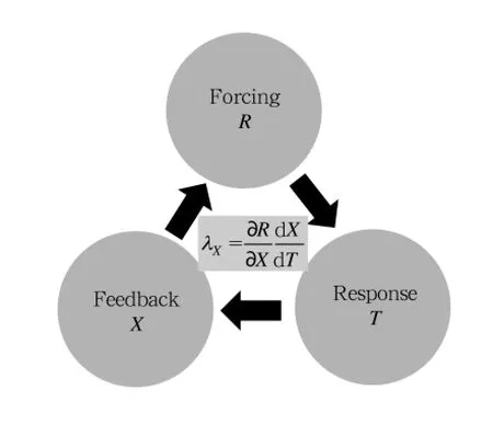
Fig.1.Schematic representation of the forcing-responsefeedback relation.λX,the feedback parameter for a certain feedback factor,means the induced perturbation of the radiative forcing at the TOA by the changes in the feedback factor per global mean surface temperature change.
Idealized radiative forcing is the net flux at the TOA without any response anywhere after the forcing agents were imposed.In such a way,the doubled CO2concentration corresponds to approximately 4.37 W m−2(Ramaswamy et al.,2001).As research progressed,climate scientists began to understand that the forcing responsible for the change in Tsis the unbalanced radiation after rapid adjustments.For example,the stratosphere can adjust to radiative equiliilibrium within one month;whereas,the changes in the troposphere,which are of greater concern,are slower and caused by the forcing after stratospheric adjustment.Taking this into consideration,the Intergovernmental Panel on Climate Change(IPCC)modified the definition of radiative forcing in its third assessment report(TAR),with the doubled CO2forcing revised to 3.71 W m−2(Ramaswamy et al.,2001).Although the above concept of forcing was preserved,other methods to calculate the forcing were proposed in the fourth IPCC report(Forster et al.,2007),including more rapid processes(but slower than the stratospheric adjustment),such as aerosol-related cloud changes(Jacob et al.,2005)and temperature adjustment in the troposphere(Hansen et al.,2005).
Multiple definitions of radiative forcing are summarized in the fifth IPCC report(AR5),including the earlier definitions outlined above.A new definition, called effective radiative forcing(ERF)was proposed. The ERF is the doubled CO2forcing at the TOA, but considers all kinds of rapid adjustments,including temperature changes in the troposphere and on land,aerosol-cloud interaction,and changes in the vertical structure of temperature and its effect on cloud (Myhre et al.,2013).The timescale of temperature change that we are concerned with is longer than the decadal scale,and up to the century scale.Hence,the ERF can better represent the forcing agents able to impact the temperature change on longer time scales (Zhang and Huang,2014).Because current understanding of the rapid adjustments is insufficient,large uncertainty is observed in model-based estimations of the ERF(2.6–4.3 W m−2;Flato et al.,2013).
The ultimate magnitude of the response is not only determined by the forcing,but also strongly influenced by various feedback processes.Stronger positive feedback leads to higher climate sensitivity,and vice versa.The forcing-response-feedback paradigm represents a cyclic interaction to a new equilibrium state(Fig.1).Next,we will review the main feedback mechanisms recognized to date.
2.1Planck feedback
Based on the Stefan-Boltzmann law,the surface heated by the radiative forcing will emit more infrared
energy outwards and reduce the net flux at the TOA. This basic negative feedback is called black-body radiation feedback or Planck feedback.Some studies have suggested that this process can be used as a reference system to measure other feedbacks,rather than being a solo feedback,because it is the simplest and most well-established relation between temperature and radiation(Roe,2009).When contributions of different processes to the change in Tsare focused upon without a reference system,the cooling effect of Planck radiation can be regarded as an important feedback (Gregory and Forster,2008;Chen et al.,2014;Pithan and Mauritsen,2014).
2.2 Water vapor feedback
Water vapor is the most important GHG in that it exerts the strongest warming effect.Based on the Clausius-Clapeyron relation,the water vapor in the atmosphere strictly depends on the temperature.Considering the short period of the atmospheric hydrological cycle(about 10 days),the water vapor should be treated as a feedback rather than forcing.The increased Tsinduced by external forcing will enhance surface evaporation and hold more water vapor in the air.More water vapor will block more outgoing radiation and increase the forcing at the TOA,which is the well-known water vapor feedback process(Held and Soden,2000;Han et al.,2015).
2.3 Lapse-rate feedback
The lapse rate of tropospheric temperature will change when the climate system warms.In the tropical regions,more water vapor condenses in the midupper troposphere and heats the local atmosphere, resulting in the warming in the upper layer being stronger than in the lower layer.This process is called moist adiabatic adjustment,in which the moist adiabatic lapse rate decreases.The warmer upper layer is conducive to the emission of more infrared radiation to space and a reduction in the forcing at the TOA.This is negative lapse-rate feedback.The warmer regions in the troposphere are usually filled with more water vapor,especially in the tropics.As a result,the positive water vapor feedback and negative lapse-rate feedback can partly cancel one another out,and the net feedback is still positive(Cess,1975;Held and Soden, 2000;Soden and Held,2006).Thus,these two closely related feedbacks are unified under the notion of water vapor-lapse-rate feedback.However,if we choose relative humidity instead of specific humidity as the feedback agent,the compensation will be substantially reduced(Held and Shell,2012;Ingram,2013).In the mid-high latitudes,warming is confined to the lower layer for a lack of moist adiabatic adjustment.The consequent positive lapse-rate feedback mainly contributes to the polar amplification phenomenon(Colman,2003;Pithan and Mauritsen,2014).
2.4Snow-ice albedo feedback
The snow cover and sea ice in the high latitudes can rapidly respond to surface warming.Melted snow and ice decrease the surface albedo and shortwave radiations reflected back to space,and increase the forcing at the TOA.This is positive snow-ice albedo feedback,which is one of the main contributors to polar amplification(Pithan and Mauritsen,2014),as shown in the earliest study on climate sensitivity(Arrhenius, 1896).
2.5Cloud feedback
The cloud response is very complex against the background of climate warming.A variety of cloud parameters,such as cloud fraction,height,particle size,phase,etc.,can all impact upon the radiative flux at the TOA.One change in a cloud attribute may bring about both positive and negative feedbacks at the same time.If the cloud fraction decreases with surface warming,increased outgoing longwave(incident shortwave)radiation will reduce(amplify)the TOA forcing,acting as a negative(positive)feedback. The sign of the net cloud feedback is then difficult to determine.The cloud at different altitudes has different radiative effects.High cloud is more opaque to longwave radiation,whereas low cloud mainly reflects shortwave radiation.As a result,both an increase in high cloud and a decrease in low cloud induced by surface warming can lead to positive feedback.In the tropics,the cloud top rises with the tropopause as the tropospheric temperature increases,resulting in positive feedback by reducing the emission of longwave
radiation.Under global warming,storm tracks shift poleward with the expansion of the Hadley circulation.As a result,the area covered by frontal cloud is reduced and heated by more solar radiation,acting as a positive feedback.Most of the models used in IPCC AR5 show that the net cloud feedback may be positive (Boucher et al.,2013).
2.6 Other feedbacks
If the air-sea CO2exchange is considered,more CO2will be released into the atmosphere from the warmer ocean by reducing the solubility,increasing the radiative forcing at the TOA.This is positive solubility feedback.Feedbacks become more complex when changes of the biosphere are involved.The response of vegetation cover to warming could change the land albedo and produce vegetation-albedo feedback(Zeng and Yoon,2009).Another example,ocean acidification due to CO2uptake may decrease the emission of dimethylsulphide by marine organisms,which is the largest natural source of atmospheric sulfur.The decrease in atmospheric sulfate will affect cloud formation and ultimately the radiative budget(Six et al., 2013).Therefore,in addition to the physical feedback mentioned above,feedbacks involving biogeochemical processes are also important.Thus,the development of earth system models that include biogeochemical cycles is at the forefront of climate modeling research (Zhou et al.,2014).
The forcing-response-feedback relation describing physical responses can be linearly expressed as
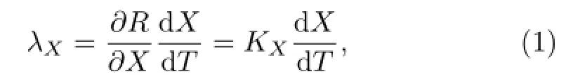
where X is a certain feedback agent,such as water vapor;R is the radiative forcing at the TOA;T is the global mean surface air temperature;KXis called the Feedback Kernel,which describes the contribution of one unit change in X to R and only depends on the radiative transfer process;dX/dT is the response of X to surface warming;and λXis the feedback parameter with respect to X.
For different feedback agents X,how to calculate the corresponding λXbased on Eq.(1)is the central issue of feedback analysis.Readers are referred to Soden et al.(2008)and Roe(2009)for a more detailed description of the feedback analysis method and Radiative Kernel approach to calculating λX.
3.Principle of estimating climate sensitivity
The estimation of climate sensitivity is based on energy conservation,

where N is the net radiative flux at the TOA;F is the radiative forcing exerted by the forcing agent;E is the increased outgoing radiation after the atmosphereearth system responds;and the positive direction is downward. To the first-order approximation,E is expressed as the linear function with respect to the change in global mean surface air temperature T′,
where λ is the net feedback parameter,the sum of all feedback components.Equations(2)and(3)are fundamental in estimating climate sensitivity based on either observation or simulation.
3.1ECS
Under a fixed 2×CO2concentration,a fully coupled ocean-atmosphere model is integrated from the pre-industrial baseline to a new equilibrium.Then, the Tsdifference between the two states is the value of ECS.However,it is not easy to reach the equilibrium state due to the expensive computational cost. As an alternative,a slab ocean model is usually coupled with the AGCM.Though the computing cost is cheap,the simplified climate system cannot introduce the effect of ocean circulation.Technically,coupling a slab ocean model with an AGCM is not easier than the development of a fully coupled model.Thus,an approximation method was proposed based on the transient state from a fully coupled model to estimate the ECS(Gregory et al.,2004).Combining Eqs.(2)and (3),the following can be obtained:

As the CO2concentration is fixed,F is a constant. Then,N can be regarded as a function with respect
to T′.By linear fitting N against T′,F at the intercept of the y-axis(T′=0)can be obtained,and the equilibrium temperature(i.e.,ECS under 2×CO2)at the intercept of the x-axis(N=0).The slope of the fitting line is λ.
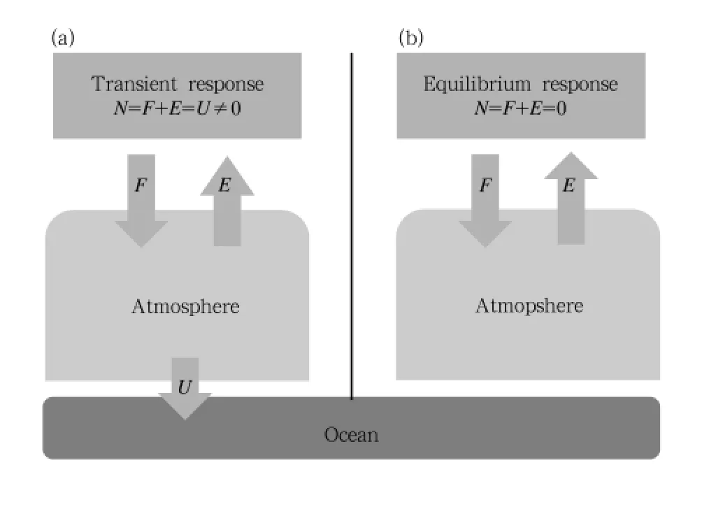
Fig.2.Schematic representation of the(a)transient response and(b)equilibrium response.N is net radiative flux at the TOA;F is radiative forcing induced by forcing factors;E is increased outgoing radiative flux of the earth system due to warming;and U denotes ocean heat uptake.For the transient response,N approximates to U, both non-zero.For the equilibrium response,E offsets F, and a new equilibrium state is reached.
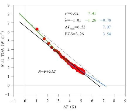
Fig.3.Relation between surface temperature change∆T and net radiative flux N at the TOA under the 4×CO2scenario.∆T and N are the differences between the abrupt 4×CO2and piControl runs.Gregory-style regression(Gregory et al.,2004)is used to estimate ECS.The outputs of the multi-model ensemble of 24 CMIP5 models are shown. The feedback parameter λ is evidently different in two response stages(roughly before and after the 20th year).
When the equilibrium is reached,the net flux N at the TOA is zero(Fig.2).ECS is expressed as

where F2×is the forcing of 2×CO2,ERF estimated based on a specific model,or 3.71 W m−2,as commonly used before;1/(−λ)is called the climate sensitivity parameter,which describes the warming induced by 1 W m−2of forcing at the TOA.
To obtain a more evident forced signal,4×CO2forcing is usually used to drive the fully coupled model. Based on the empirical relation between CO2concentration and radiative forcing(Myhre et al.,1998),the forcing of 4×CO2is exactly twice that of 2×CO2.Assuming λ is unchanged,ECS is half the equilibrium temperature estimated from the 4×CO2scenario.Figure 3 shows an application of Gregory-style regression to obtain ECS using the average of 24 CMIP5 models.The response in the models shows two stages:a fast response in the first 20 years(green line)and a slow response later on(blue line),corresponding to different λ(Chen et al.,2014).The mean λ estimated by the ERF and ECS based on the two stages(dashed black line)is similar to λ calculated by using the whole period(solid black line).ECS estimated only by the slow response stage(the last 130 years)is 0.3 K higher than that derived from the whole period.
Besides model output,observational data can also be used to estimate ECS in nature.However,in the real world,F evolves with time.Based on Eq.(4), we should know the time series of F contributed from GHGs,aerosols,land use,solar perturbation,volcano activity,and so on.The unbalanced flux N at the TOA and the surface temperature change T′should also be known.Then,we can fit(N−F)against T′to obtain the value of λ and subsequently use Eq.(5) to estimate ECS(Forster and Gregory,2006).
3.2TCR and TCRE
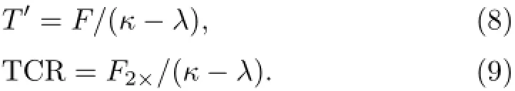
The TCR measures the sensitivity to CO2forcing in the non-equilibrium state.Besides the feedback,the TCR is affected by the ocean heat uptake(OHU)(Fig. 2).For the transient response,the energy conservation
is also satisfied,so we have

where U is the OHU,equal to the net flux at the TOA. Assuming the timescale of OHU is much longer than that of the Tsresponse,U can be approximated as the first-order relation with T′,

where κ is the efficiency of OHU with a positive value. This linear approximation assumes that the ocean has infinite heat capacity and the OHU is regarded as one kind of negative feedback,which is applicable to the forcing of a moderate increasing scenario(Gregory and Forster,2008).Combining Eqs.(6)and(7),we obtain
It is evident that a strong OHU can lead to a small TCR.
Based on the definition of TCR,in practice,the value of TCR is calculated by using the change of Ts, a 20-yr mean state centered on the time of CO2doubling under the 1%yr−1increasing scenario relative to the pre-industrial baseline.Using the same experiment,we can calculate the cumulative CO2emissions in the atmosphere Ce(unit:Pg C)before the CO2concentration is doubled.Then,TCRE is expressed as

The units of TCRE are usually converted to 10−3K Pg C.The emissions-driven earth system model is another tool that can be used to estimate TCR.The difference from the conventional model is that the value of Ceis determined by the carbon cycle and related feedbacks, which may vary across models.Thus,TCRE is the regression coefficient by fitting Tsagainst the cumulative CO2emissions(Collins et al.,2013).
4.Uncertainty in climate sensitivity
From IPCC TAR to AR5,extensive studies using paleoclimatic proxy data,historical instrumental observations and multi-model simulations,have not reduced the uncertainty of the ECS.The newly suggested possible range is 1.5–4.5 K,the same as the Charney sensitivity obtained in 1979(Charney et al., 1979).Besides,a diverse range of results are seen in different studies(Gregory et al.,2002;Forster and Gregory,2006;Andrews et al.,2012;Olson et al.,2012; Rohling et al.,2012;Masters,2014).It is also believed that the relation between the feedback and ECS intrinsically determines the uncertainty(Roe and Baker, 2007).
From Eq.(5),we have
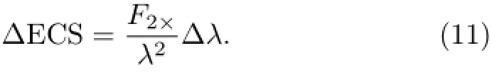
This shows the relation between the uncertainties of λ and ECS under the linearization assumption.If λ is small,∆ECS will be large following one unit change of∆λ.This means that the uncertainty of ECS is inevitably large if ECS itself is not small enough,which results in the upper limit of the probability being hard to constrain.It should be noted that these results are derived from the assumption of linear feedback. Therefore,it is still controversial in understanding the relation between ECS and feedbacks(Roe and Armour,2011).
The uncertainties of ECS estimated by models mainly come from feedback processes,especially cloud feedback,which contributes about 70%of inter-model variance of ECS.The shortwave feedback of low cloud in the tropical and subtropical regions(including shallow convective cloud and stratocumulus)is highly uncertain(Randall et al.,2007;Klocke et al.,2011;Vial et al.,2013).The uncertainty of observation-based estimations of ECS comes from the observational data themselves,such as the net flux at the TOA,the forcing exerted by a variety of agents,and the OHU.Although ECS is the sensitivity to the CO2concentration,the observed change in Tsis the result of multiple forcing agents(Ma et al.,2005).Hence,to accurately estimate the climate feedback,the forcing from all the agents should be known.Besides the GHG forcing, aerosol is another important forcing agent that can exert forcing directly(the direct effect)and also impact the radiative budget via interactions with cloud
(the indirect effect).The difficulty in estimating the aerosol forcing adds more uncertainty to the accurate estimation of the ECS/TCR.
TheOHU playsan importantrolein the TCR/TCRE.A strong OHU delays the warming (Zhao and Shi,1995;Stouffer et al.,2006).The simulation of eddy mixing intensity in ocean models can significantly affect the OHU in the vertical profile. Strong mixing in the Southern Ocean favors more heat taken up by the ocean,which is further transported into the deep ocean through the meridional overturning circulation(Zhang and Vallis,2013).Large divergence in the spatial distribution of the OHU across models has been observed.Two typical distributions are prominent in the zonally mean pattern:highlatitude OHU and low-latitude OHU,and these have different influences on the global warming.Following a more effective high-latitude OHU,weaker warming is witnessed(Winton et al.,2010;Rose et al.,2014). If the carbon cycle is considered,the increasing rate of the cumulative CO2emissions is closely related to the carbon sources and sinks on land and in the ocean.The uncertainties in the ecological processes and the interactions with temperature,precipitation, and ocean circulation,can further impact the magnitude of the TCRE(Gillett et al.,2013).
5.Relationship between the 2℃threshold and climate sensitivity
The 2℃threshold issue is of wide concern among the public and research community.The 2℃warming of Tsabove the pre-industrial level is considered as a threshold that indicates dangerous anthropogenic interference(Mann,2009).Given the same radiative forcing and OHU,a larger ECS will shorten the time that it takes to reach a 2℃warming.If ECS is relatively large,the aim of an ultimate warming below 2℃requires a small forcing(CO2concentration),which puts greater stress on emission reduction for human society.The issue can be understood based on the forcing-response relation.
Based on Eq.(4),the ultimate equilibrium temperature∆T is proportional to the forcing F.Assuming constant feedback λ,we obtain
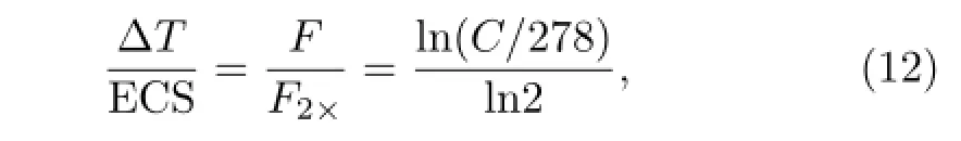
where C(ppm)is the current concentration of CO2, which is assumed to remain unchanged;278 ppm is the pre-industrial reference CO2concentration.The CO2concentration C can be expressed as a function of equilibrium warming∆T and ECS,

The relationship between C and ECS given at∆T =1.5℃(blue line),2℃(black line),and 3℃(magenta line)is shown in Fig.4.The range of ECS is from the IPCC estimation,i.e.,1.5–4.5 K.When∆T=2℃and the value of ECS is near the median of the range (about 3 K,50%probability higher or lower),the corresponding CO2concentration is about 450 ppm.This forms the basis of the statement that the atmospheric CO2concentration should not exceed 450 ppm if the warming is intended to be below the 2℃ threshold (Schneider et al.,2007;Calvin et al.,2009;Wang et al.,2013;Oppenheimer et al.,2014).
It should be noted that the uncertainty in ECS has a substantial impact on the CO2concentration under a certain temperature target.If ECS is 1.5 K, the CO2concentration can be as large as 700 ppm (Fig.4).However,based on current knowledge,the probability of an ECS below 1.5 K is very small(less than 0.05;Stocker et al.,2013).That is why Mann (2014)emphasized the importance and urgency of reducing GHG emissions,although we have experienced
a flat warming period referred to as the global warming hiatus during the last decade.
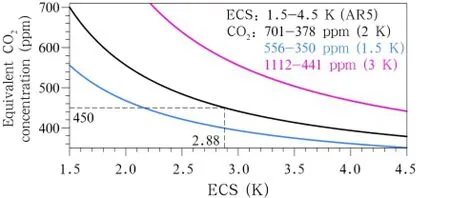
Fig.4.Relationship between the equivalent CO2concentration and ECS constrained by a certain warming threshold.The range of ECS is from the new estimation in IPCC AR5.The curves under the 1.5℃(blue),2℃(black),and 3℃(magenta)threshold are shown.For the 2℃threshold, the corresponding equivalent CO2concentration is about 450 ppm when ECS is the median estimated value.
6.Research prospects
The history of research on climate sensitivity can be traced back 100 years.Following the increase in observational data,the development of fully coupled climate system or even earth system models,and the improvement of approaches to feedback analysis,our understandings on the issue have greatly improved. Nevertheless,there remain a great number of challenges.For example,high-quality observational data have too short history to detect the climate change signal,especially in the Southern Ocean where the OHU is substantially large.In addition,the parameterization processes in current state-of-the-art climate models are far from perfect.This further reduces the reliability and limits the application of model output.The difficulty in reducing the uncertainty of climate sensitivity can be either due to the intrinsic climate system or the deficiency of our current knowledge.Based on our review of recent progress in this field,the following research priorities are recommended to the climate sensitivity research community,in particular the Chinese community where the contribution of climate sensitivity studies remains weak.
6.1 Nonlinear interaction of feedbacks
Linear feedback analysis is a mature method.The Radiative Kernel approach based on linear feedback analysis can provide spatial distribution information on different feedback processes.However,large gaps between the sum of individual feedbacks and total feedback are found in many models,indicating that strong nonlinear interactions are non-negligible(Via et al.,2013).The climate sensitivity is determined by feedback.Therefore,the interactions among different feedback processes should be highlighted in future research.
6.2 Constraining climate sensitivity by combining new observations and model development
One precondition for reliable climate sensitivity in a model is that the historical climate change should be reasonably reproduced by the model,such as the warming trend in the 20th century.Many models still show limitations in this regard(Zhou and Yu, 2006;Zhou et al.,2013).The uncertainty of a climate model's sensitivity could be reduced if the model has been sufficiently constrained by observations(Jackson et al.,2008).Cloud-related convection is one important source of uncertainty in climate sensitivity(Sherwood et al.,2014).It is necessary to improve the spatiotemporal resolution of cloud and convection monitoring on the global scale,to promote understanding of the interactions between cloud,convection and largescale circulation,and properly parameterize these processes in climate models(Stevens and Bony,2013).In addition,it remains a great challenge for climate models to simulate the abrupt change recorded in paleoclimatic record,which is a strict criterion to test the performance of climate models(Wang et al.,2013).
6.3 Estimating earth system sensitivity
Under the concept of traditional physical climate, the focus of climate sensitivity research is the forcingresponse-feedback process following an increase of atmospheric CO2.However,the responses of land and ocean carbon repositories are not taken into account. In nature,the carbon cycle,including biological effects,can further feed back to the increasing atmospheric CO2concentration and surface warming.This kind of process can influence the change in Tsfrom the decadal to the millennial timescales,and impact the estimation of ECS.The carbon cycle and related feedbacks determine the increasing rate of cumulative CO2emissions,adding further uncertainty to the TCRE. Thus,more effort is needed in terms of estimating the earth system sensitivity,and developing an optimal emission path using the concept of TCRE.
Acknowledgments.We would like to thank the two anonymous reviewers for their constructive suggestions and comments,which helped in improving the paper.
Andrews,T.,J.M.Gregory,M.J.Webb,et al.,2012: Forcing,feedbacks and climate sensitivity in CMIP5 coupled atmosphere-ocean climate models.Geophys. Res.Lett.,39,L09712.
Arrhenius,S.,1896:On the influence of carbonic acid in the air upon the temperature of the ground.Philos. Mag.,41,237–276.
Boucher,O.,D.Randall,P.Artaxo,et al.,2013:Clouds and aerosols.Climate Change 2013:The Physical Science Basis.Stocker,T.F.,D.H.Qin,G.-K. Plattner,et al.,Eds.,Cambridge University Press, Cambridge,United Kingdom and New York,USA, 1535 pp.
Calvin,K.V.,J.A.Edmonds,B.Bond-Lamberty,et al., 2009:2.6:Limiting climate change to 450 ppm CO2equivalent in the 21st century.Energ.Econ.,31, S107–S120.
Cess,R.D.,1975:Global climate change:An investigation of atmospheric feedback mechanisms.Tellus, 27,193–198.
Charney,J.,A.Arakawa,D.J.Baker,et al.,1979:Carbon dioxide and climate:A scientific assessment. Report of an Ad Hoc Study Group on Carbon Dioxide and Climate. National Academy of Sciences Press,Washington D.C.,22 pp.
Chen Xiaolong,Zhou Tianjun,and Guo Zhun,2014:Climate sensitivities of two versions of FGOALS model to idealized radiative forcing.Sci.China(Earth Sci.),57,1363–1373.
Collins,M.,R.Knutti,J.Arblaster,et al.,2013:Longterm climate change:Projections,commitments and irreversibility.Climate Change 2013:The Physical Science Basis. Stocker,T.F.,D.H.Qin,G.-K. Plattner,et al.,Eds.,Cambridge University Press, Cambridge,United Kingdom and New York,USA, 1535 pp.
Colman,R.,2003:Seasonal contributions to climate feedbacks.Climate Dyn.,20,825–841.
Cubasch,U.,G.Meehl,G.J.Boer,et al.,2001:Projections of future climate change.Climate Change 2001:The Scientific Basis.Houghton,J.T.,Y.H. Ding,D.J.Griggs,et al.,Eds.,Cambridge University Press,Cambridge,United Kingdom and New York,USA,881 pp.
Danabasoglu,G.,and P.R.Gent,2009:Equilibrium climate sensitivity:Is it accurate to use a slab ocean model?J.Climate,22,2494–2499.
Flato,G.,J.Marotzke,B.Abiodun,et al.,2013:Evaluation of climate models.Climate Change 2013:The Physical Science Basis.Stocker,T.F.,D.H.Qin, G.-K.Plattner,et al.,Eds.,Cambridge University Press,Cambridge,United Kingdom and New York, USA,1535 pp.
Forster,P.M.F.,and J.M.Gregory,2006:The climate sensitivity and its components diagnosed from earth radiation budget data.J.Climate,19,39–52.
Forster,P.,V.Ramaswamy,P.Artaxo,et al.,2007: Changes in atmospheric constituents and in radiative forcing.Climate Change 2007:The Physical Science Basis.Solomon,S.,D.H.Qin,M.Manning, et al.,Eds.,Cambridge University Press,Cambridge, United Kingdom and New York,USA,996 pp.
Gillett,N.P.,V.K.Arora,D.Matthews,et al.,2013: Constraining the ratio of global warming to cumulative CO2emissions using CMIP5 simulations.J. Climate,26,6844–6858.
Goodwin,P.,R.G.Williams,and A.Ridgwell,2015: Sensitivity of climate to cumulative carbon emissions due to compensation of ocean heat and carbon uptake.Nat.Geosci.,8,29–34.
Gregory,J.M.,R.J.Stouffer,S.C.B.Raper,et al., 2002:An observationally based estimate of the climate sensitivity.J.Climate,15,3117–3121.
Gregory,J.M.,W.J.Ingram,M.A.Palmer,et al., 2004:A new method for diagnosing radiative forcing and climate sensitivity.Geophys.Res.Lett.,31, L03205.
Gregory,J.M.,and P.Forster,2008:Transient climate response estimated from radiative forcing and observed temperature change.J.Geophys.Res.,113, D23105.
Han Bo,L¨u Shihua,et al.,2015:Connection between atmospheric latent energy and energy fluxes simulated by nine CMIP5 models.J.Meteor.Res.,29, 412–431.
Hansen,J.,A.Lacis,D.Rind,et al.,1984:Climate sensitivity:Analysis of feedback mechanisms.Climate Processes and Climate Sensitivity.Hansen,J. E.,and T.Takahashi,Eds.,American Geophysical Union,Washington D.C.,130–163.
Hansen,J.,M.Sato,R.Ruedy,et al.,2005:Efficacy of climate forcings.J.Geophys.Res.,110,D18104.
Held,I.M.,and B.J.Soden,2000:Water vapor feedback and global warming.Annu.Rev.Energy Environ., 25,441–475.
Held,I.M.,and K.M.Shell,2012:Using relative humidity as a state variable in climate feedback analysis. J.Climate,25,2578–2582.
Ingram,W.,2013:A new way of quantifying GCM water vapour feedback.Climate Dyn.,40,913–924.
IPCC,1990:Climate Change:The IPCC Scientific Assessment. Houghton,J.T.,G.J.Jenkins,J.J.
Ephraums,Eds.,Cambridge University Press,Cambridge,United Kingdom and New York,USA,365 pp.
Jackson,C.S.,M.K.Sen,G.Huerta,et al.,2008:Error reduction and convergence in climate prediction.J. Climate,21,6698–6709.
Jacob,D.J.,R.Avissar,G.C.Bond,et al.,2005:Radiative Forcing of Climate Change:Expanding the Concept and Addressing Uncertainties. The National Academies Press,Washington D.C.,207 pp.
Klocke,D.,R.Pincus,and J.Quaas,2011:On constraining estimates of climate sensitivity with present-day observations through model weighting.J.Climate, 24,6092–6099.
Li,C.,J.-S.Von Storch,and J.Marotzke,2013:Deepocean heat uptake and equilibrium climate response. Climate Dyn.,40,1071–1086.
Ma Xiaoyan,Shi Guangyu,Guo Yufu,et al.,2005:Radiative forcing by greenhouse gases and sulfate aerosol. Acta Meteor.Sinica,63,41–48.(in Chinese)
Manabe,S.,and R.F.Strickler,1964:Thermal equilibrium of the atmosphere with a convective adjustment.J.Atoms.Sci.,21,361–385.
Manabe,S.,and R.T.Wetherald,1967:Thermal equilibrium of the atmosphere with a given distribution of relative humidity.J.Atoms.Sci.,24,241–259.
Manabe,S.,and R.T.Wetherald,1975:The effects of doubling the CO2concentration on the climate of a general circulation model.J.Atoms.Sci.,32,3–15. Mann,M.E.,2009:Defining dangerous anthropogenic interference.Proc.Nat.Acad.Sci.USA,106, 4065–4066.
Mann,M.E.,2014:False hope.Sci.Am.,310,78–81.
Masters,T.,2014:Observational estimate of climate sensitivity from changes in the rate of ocean heat uptake and comparison to CMIP5 models.Climate Dyn.,42,2173–2181.
Matthews,H.D.,N.P.Gillet,P.A.Stott,et al.,2009: The proportionality of global warming to cumulative carbon emissions.Nature,459,829–832.
Myhre,G.,E.J.Highwood,K.P.Shine,et al.,1998: New estimates of radiative forcing due to well mixed greenhouse gases.Geophys.Res.Lett.,25,2715–2718.
Myhre,G.,D.Shindell,F.-M.Br´eon,et al.,2013:Anthropogenic and natural radiative forcing.Climate Change 2013:The Physical Science Basis.Stocker, T.F.,Qin Dahe,G.-K.Plattner,et al.,Eds.,Cambridge University Press,Cambridge,United Kingdom and New York,USA,1535 pp.
Olson,R.,R.Sriver,M.Geos,et al.,2012:A climate sensitivity estimate using Bayesian fusion of instrumental observations and an Earth System model.J. Geophys.Res.,117,D04103.
Oppenheimer,M.,M.Campos,R.Warren,et al.,2014: Emergent risks and key vulnerabilities. Climate Change 2014:Impacts,Adaptation,and Vulnerability.Part A:Global and Sectoral Aspects.Field, C.B.,V.R.Barros,D.J.Dokken,et al.,Eds., Cambridge University Press,Cambridge,United Kingdom and New York,USA,1820 pp.
Pithan,F.,and T.Mauritsen,2014:Arctic amplification dominated by temperature feedbacks in contemporary climate models.Nat.Geosci.,7,181–184.
Ramaswamy,V.,O.Boucher,J.Haigh,et al.,2001:Radiative forcing of climate change.Climate Change 2001:The Scientific Basis.Houghton,J.T.,Y.H. Ding,D.J.Griggs,et al.,Eds.,Cambridge University Press,Cambridge,United Kingdom and New York,USA,881 pp.
Randall,D.A.,R.A.Wood,S.Bony,et al.,2007:Climate models and their evaluation.Climate Change 2007:The Physical Science Basis.Solomon,S.,D. H.Qin,M.Manning,et al.,Eds.,Cambridge University Press,Cambridge,United Kingdom and New York,USA,996 pp.
Roe,G.,2009:Feedbacks,timescales,and seeing red. Annu.Rev.Earth Planet Sci.,37,93–115.
Roe,G.H.,and M.B.Baker,2007:Why is climate sensitivity so unpredictable?Science,318,629–632.
Roe,G.H.,and K.C.Armour,2011:How sensitive is climate sensitivity?Geophys.Res.Lett.,38,L14708.
Rohling,E.J.,A.Sluijs,H.A.Dijkstra,et al.,2012: Making sense of palaeoclimate sensitivity.Nature, 491,683–691.
Rose,B.E.J.,K.C.Armour,D.S.Battisti,et al.,2014: The dependence of transient climate sensitivity and radiative feedbacks on the spatial pattern of ocean heat uptake.Geophys.Res.Lett.,41,1071–1078.
Schneider,S.H.,S.Semenov,A.Patwardhan,et al., 2007: Assessing key vulnerabilities and the risk from climate change.Climate Change 2007:Impacts,Adaptation and Vulnerability.Solomon,S., D.H.Qin,M.Manning,et al.,Eds.,Cambridge University Press,Cambridge,United Kingdom and New York,USA,976 pp.
Sherwood,S.C.,S.Bony,and J.-L.Dufresne,2014: Spread in model climate sensitivity traced to atmospheric convective mixing.Nature,505,37–42.
Shi Guangyu,1991:Radiative forcing and greenhouse effect due to the atmospheric trace gases.Sci.China (Ser.B),35,217–229.
Six,K.D.,S.Kloster,T.Ilyina,et al.,2013:Global warming amplified by reduced sulphur fluxes as a result of ocean acidification.Nat.Climate Change, 3,975–978.
Soden,B.J.,and I.M.Held,2006:An assessment of climate feedbacks in coupled ocean-atmosphere models.J.Climate,19,3354–3360.
Soden,B.J.,I.M.Held,R.Colman,et al.,2008:Quantifying climate feedbacks using radiative kernels.J. Climate,21,3504–3520.
Stevens,B.,and S.Bony,2013:What are climate models missing?Science,340,1053–1054.
Stocker,T.F.,D.H.Qin,G.-K.Plattner,et al.,2013: Technical summary. Climate Change 2013:The Physical Science Basis.Stocker,T.F.,D.H.Qin, G.-K.Plattner,et al.,Eds.,Cambridge University Press,Cambridge,United Kingdom and New York, USA,1535 pp.
Stouffer,R.J.,and S.Manabe,1999:Response of a coupled ocean-atmosphere model to increasing atmospheric carbon dioxide:Sensitivity to the rate of increase.J.Climate,12,2224–2237.
Stouffer,R.J.,J.Russell,and M.J.Spelman,2006:Importance of oceanic heat uptake in transient climate change.Geophys.Res.Lett.,33,L17704.
Vial,J.,J.-L.Dufresne,and S.Bony,2013:On the interpretation of inter-model spread in CMIP5 climate sensitivity estimates.Climate Dyn.,41,3339–3362.
Wang Mingxing,Zhang Renjian,and Zheng Xunhua, 2000:Sources and sinks of greenhouse gases.Climatic Environ.Res.,5,75–79.(in Chinese)
Wang Shaowu,Luo Yong,Zhao Zongci,et al.,2012:Equilibrium climate sensitivity.Adv.Climate Change Res.,8,232–234.(in Chinese)
Wang Shaowu,Luo Yong,Zhao Zongci,et al.,2013:The Sciences of Global Warming.China Meteorological Press,Beijing,205 pp.(in Chinese)
Winton,M.,K.Takahashi,and I.M.Held,2010:Importance of ocean heat uptake efficacy to transient climate change.J.Climate,23,2333–2344.
Zeng,N.,and J.Yoon,2009:Expansion of the world's deserts due to vegetation-albedo feedback under global warming.Geophys.Res.Lett.,36,L17401.
Zhang Hua and Huang Jianping,2014:Interpretation of the IPCC Fifth Assessment Report on anthropogenic and natural radiative forcing.Adv.Climate Change Res.,10,40–44.(in Chinese)
Zhang,Y.,and G.K.Vallis,2013:Ocean heat uptake in eddying and non-eddying ocean circulation models in a warming climate.J.Phys.Oceanogr.,43, 2211–2229.
Zhao Fengsheng and Shi Guangyu,1995:A study of the transient and time-dependent greenhouse gasinduced climate change.Acta Geogra.Sinica,50, 430–438.(in Chinese)
Zhou Tianjun,Song Fengfei,and Chen Xiaolong,2013: Historical evolution of global and regional surface air temperature simulated by FGOALS-s2 and FGOALS-g2:How reliable are the model results? Adv.Atmos.Sci.,30,638–657.
Zhou Tianjun,Wang Shaowu,and Zhang Xuehong,1998: Proceeding of modelling studies on the stability and variability of the thermohaline circulation. Adv. Earth Sci.,13,334–343.(in Chinese)
Zhou Tianjun,Wang Shaowu,and Zhang Xuehong,2000: Comments on the role of thermohaline circulation in global climate system.Adv.Earth Sci.,15,654–660.(in Chinese)
Zhou,T.J.,and R.C.Yu,2006:Twentieth-century surface air temperature over China and the globe simulated by coupled climate models.J.Climate, 19,5843–5858.
Zhou Tianjun,Zou Liwei,Wu Bo,et al.,2014:Development of earth/climate system models in China: A review from the coupled model intercomparison project perspective.J.Meteor.Res.,28,762–779.
:Zhou Tianjun and Chen Xiaolong,2015:Uncertainty in the 2℃warming threshold related to climate sensitivity and climate feedback.J.Meteor.Res.,29(6),884–895,
10.1007/s13351-015-5036-4.
Supported by the Strategic Priority Research Program of the Chinese Academy of Sciences(XDA05110300)and National Natural Science Foundation of China(41330423).
∗Corresponding author:chenxiaolong@mail.iap.ac.cn.
©The Chinese Meteorological Society and Springer-Verlag Berlin Heidelberg 2015
(Received May 19,2015;in final form October 15,2015)
 Journal of Meteorological Research2015年6期
- Journal of Meteorological Research的其它文章
- Advances in Research on Atmospheric Energy Propagation and the Interactions between Different Latitudes
- Asymmetric Features for Two Types of ENSO
- ENSO-Independent Contemporaneous Variations of Anomalous Circulations in the Northern and Southern Hemispheres:The Polar-Tropical Seesaw Mode
- Seasonal Inhomogeneity of Soot Particles over the Central Indo-Gangetic Plains,India:Influence of Meteorology
- Effect of Urbanization on the Urban Meteorology and Air Pollution in Hangzhou
- Role of a Meso-γ Vortex in Meiyu Torrential Rainfall over the Hangzhou Bay,China:An Observational Study