基于第一性原理量子输运模拟的并行计算
2015-12-31 21:46张若兴侯士敏国家核电技术公司北京软件技术中心国家能源核电软件重点实验室北京0009北京大学电子学系纳米器件物理与化学教育部重点实验室北京0087
计算物理 2015年6期
张若兴, 侯士敏, 丑 强(.国家核电技术公司北京软件技术中心国家能源核电软件重点实验室,北京 0009;.北京大学电子学系纳米器件物理与化学教育部重点实验室,北京 0087)
基于第一性原理量子输运模拟的并行计算
张若兴1, 侯士敏2, 丑 强1
(1.国家核电技术公司北京软件技术中心国家能源核电软件重点实验室,北京 100029;
2.北京大学电子学系纳米器件物理与化学教育部重点实验室,北京 100871)
为了解决基于第一性原理分析计算大尺度量子输运体系时遇到的耗时长久问题,挖掘密度泛函理论与非平衡格林函数相结合方法(DFT+NEGF方法)在自洽迭代过程中的计算热点,就计算电子密度矩阵时的能量点积分和计算格林函数时的矩阵求逆/乘法运算提出MPI/OpenMP并行计算方案.能量点积分采用MPI多进程并行方案,在数据初始化时需要将稀疏矩阵和积分能量点依照轮询调度算法分配给各进程.矩阵求逆/乘法的并行化既可调用ScaLAPACK子程序实现又可调用Intel MKL数学库中的OpenMP多线程加速函数实现.由于不同能量点计算的独立性,能量点积分采用的MPI并行计算获得近乎线性的加速比曲线.由于OpenMP多线程并行采用的是基于共享内存的数据交换机制以及线程间切换通信开销小,矩阵求逆/乘法运算的OpenMP并行实现在计算效率上要优于而在程序的可扩展性上要劣于MPI多进程并行实现.
第一性原理计算;密度泛函理论;格林函数;MPI;并行计算
0 引言
进入量子领域的电子器件不再遵从传统的物理规律而是具有显著的量子效应和电导涨落特性[1],因此探索下一代电子器件的发展方向和研究它们的导电机理成为人们关注的焦点[2-3].在此方面,基于量子力学的第一性原理计算要比实验研究更有优势,因为理论研究可以低成本地模拟各种构型的量子器件并且就它们表现出来的电子输运特性给出物理解释.由于量子输运体系是无限大非周期的开放体系,在计算化学和凝聚态物理领域中被广泛应用的处理孤立体系或者周期体系的基态密度泛函理论并不是直接适用的[4].Meir 和Wingreen于1992年在Keldysh的非平衡格林函数理论的基础上给出了普适的电流计算公式[5-6],然而公式中代表能量和相位弛豫的非弹性输运贡献的电子自能项又往往是很难获得的.所以后续发展了一种近似处理方法:用密度泛函理论[7-8](Density Functional Theory,DFT)中的交换关联能代替非平衡格林函数[5,9-11](Non-Equilibrium Green’s Function,NEGF)中的电子相互作用自能.此方法就是被广泛采用的DFT 与NEGF相结合的方法,记作DFT+NEGF方法.简言之,在采用局域原子轨道基组和电极边界满足屏蔽近似的条件下,不可计算的开放体系分为可以进行传统DFT计算的周期电极部分和带有电极边界修正的有限大小的扩展分子部分[12-13].
在实验上,一个单分子结的体系一般具有几十纳米甚至几百纳米大小的尺度[14-16],组成多分子器件电路后势必将有更大的规模.因此,需要解决的一个关键问题是如何有效地提高计算效率,以使之能够处理较大体系的输运问题.基于多核CPU的OpenMP多线程并行计算和基于多台物理机的集群MPI多进程并行计算为加速DFT+NEGF自洽迭代计算指明了一个发展方向.事实上,基于第一性原理研究量子输运的商业软件Atomistix ToolKit[17]、开源软件Smeagol[18]都已实现了OpenMP和MPI并行计算.然而,这些软件更关注的是功能实现而非并行效率优化,例如Smeagol的MPI并行加速只是针对积分能量点实现的,一旦CPU总核数超过积分能量点个数会造成CPU资源的严重浪费.本文工作的意义在于不仅在前人研究的基础上实现了量子输运计算软件,还重新审视并设计了软件中的MPI/OpenMP混合并行算法,实现了比Smeagol软件更细粒度、更优化的并行计算.
1 DFT+NEGF计算流程
基于DFT+NEGF框架的量子输运计算流程如图1所示.我们需要先选取恰当的基函数和赝势,然后猜测一个初始的密度矩阵,一般取电子占据每个原子的基态作为初始猜测.对于电极,我们利用周期体系的DFT计算得到电极原胞的哈密顿量矩阵、密度矩阵和电极自能矩阵.对于扩展分子,先由给定的基函数和赝势可以计算出动能和原子核的电势,这两部分在自洽计算中不会变化.在得到扩展分子和电极的哈密顿量之后,对于每一个给定的能量,我们都可以计算出自能和扩展分子的格林函数,然后对能量积分得到密度矩阵.如果这个密度矩阵与输入的密度一样,则自洽计算成功,否则将新的密度矩阵继续代入上面的循环,计算哈密顿矩阵和下一步的密度矩阵,直到收敛为止.

图1 基于DFT+NEGF框架的量子输运计算的主流程Fig.1 Main flow of quantum transport calculations based on DFT+NEGF framework
在DFT+NEGF框架下,由于采用了局域原子轨道基组和屏蔽近似,两端量子器件的开放体系可以分割成三个典型部分,如图2所示.扩展分子的格林函数可表示为

其中ΣL和ΣR分别代表了左、右电极作为半周期边界条件对扩展分子的哈密顿矩阵的微扰,我们称之为电极自能矩阵.无论输运体系是否处于平衡状态,扩展分子的电子密度矩阵在数学上均表达为

其中扩展分子的小于格林函数在左、右电极费米能级相同的平衡状态下可写为

在左、右电极费米能级不相同的非平衡状态下可写为

GR和GA、ΓL和ΓR、AL和AR、μL和μR分别是扩展分子的推迟格林函数和超前格林函数、左右电极的展宽函数、扩展分子的谱函数中与左电极和右电极相耦合的部分、左右电极的费米能级.

图2 两端量子器件开放体系的典型划分Fig.2 Typical division of a two-end quantum transport device
2 计算热点分析
从图2可知,鉴于周期电极的DFT计算和量子输运结果分析都各执行一遍,量子输运计算的热点在于扩展分子哈密顿量矩阵H和电子密度矩阵ρ之间的自洽迭代计算.H的计算量主要在于对体系电子-电子库仑势的计算,利用快速傅立叶变换技术可以有效地将这一部分的计算量减小到O(N log N)的量级;ρ的计算量主要在于求格林函数时矩阵求逆操作(见式(1))和求电子密度矩阵时的能量积分操作(见式(2)),其计算量是O(N3),N是量子输运体系的尺度大小[19].因此,接下来我们关注的是自洽迭代过程中扩展分子格林函数和电子密度矩阵的求解.
2.1 计算格林函数矩阵
根据式(1),获知格林函数矩阵实际上是单纯的矩阵求逆操作.通用线性代数软件包 (Linear Algebra PACKage,LAPACK)提供的矩阵求逆算法是通过LU分解和回代过程两个步骤来进行的,其计算量是O (N3),也就是说每当计算体系增大一倍,求逆计算以及由此导致的NEGF计算的计算量就增大8倍.这大大限定了我们计算的体系大小.在实际计算中,由于采用了局域轨道基组,当原子之间达到一定的距离以后,它们的基组之间将没有任何重叠.这就导致求扩展分子格林函数时被求逆矩阵z S-H-ΣL-ΣR是非常稀疏的.利用这一稀疏的性质可以有效地提高求逆的速度.可以证明,对于一个带状对角的稀疏矩阵,LU分解得到的矩阵具有和原矩阵相同的稀疏程度,从而使得LU分解的计算量从原来的O(N3)降到O(N).然而在输运计算的体系中,格林函数矩阵往往不具有稀疏性,这使得回代过程的计算量仅由O(N3)降到O (N2).因此,基于稀疏矩阵的LAPACK直接求逆算法最终是个O(N2)计算量的算法[20].

图3 非平衡态下求电子密度矩阵的能量积分路径(Ceq为平衡部分的环路积分,Lne为非平衡部分贴近实轴的积分路径,Cne为非平衡部分的环路积分.)Fig.3 Energy integral path in calculating non-equilibrium electron densitymatrix(Ceqis for the equilibrium division,Lneand Cneare for the non-equilibrium divisions along the real axis and off the real axis.)
2.2 计算电子密度矩阵
实际上,把基组表象的电子密度矩阵表示成对应空间的谱函数按照费米分布填充后再对能量积分的形式,是非常形象和直观的.只不过,因为小于格林函数在能量域内可能存在大量尖峰而且费米分布函数在费米能级对应的虚轴上存在奇点,所以利用式(2)积分求电子密度矩阵在数学实现上是一项非常有技巧性的工作.简单地说,平衡态下的电子密度矩阵可以利用复平面内的环路积分和留数定理得到,而非平衡态下的电子密度矩阵积分可以通过公式变形分成两部分:利用环路积分的平衡部分和处在左、右电极的费米能级之间贴近实轴积分的非平衡部分[20-23],非平衡态下的双路径积分见图3所示.变形积分路径的一个最大的好处在于我们可以用一个非常稀疏的积分网格点划分来得到一个相对精确的积分结果,因为格林函数在远离实轴的区域变得非常的平滑.数学上有很多成熟的算法来处理这一数值积分问题.目前,基于DFT+NEGF的量子输运计算软件多数采用Gaussian积分算法[24].不同的是,我们采用了Gauss-Kronrod积分算法[24],特征是对积分路径上不同平滑程度的区域采用不同疏密的函数取值点使得格林函数的积分更加有效率.图4给出了金-吡啶-金分子结量子输运体系的推迟格林函数在上半复能量域上的平滑程度以及采用Gauss-Kronrod积分的自适应能量取点分布.可见,在靠近实轴和费米能级的区域,算法自动给出了更密的函数取点.

图4 金-吡啶-金分子结量子输运体系Fig.4 Au-pyridine-Au molecular junction
3 并行计算方案
正如2.1节所述,因为采用了局域的原子轨道基组,为了节省内存和加快矩阵运算我们对稀疏形式的大规模矩阵采用压缩存储.如图5所示,在并行计算方案中,考虑到各进程间的负载均衡和MPI通信开销,应选择合适的块大小(BlockSize)将稀疏矩阵按照轮询调度算法(Round-Robin Scheduling)分配给所有进程.若BlockSize过小则MPI进程间通信频繁,开销大;若BlockSize过大则有的进程可能分配不到计算任务,负载均衡差.另外,每个进程维护着压缩存储矩阵的本地索引表并且能够还原成稀疏矩阵中对应非零元素的索引.

图5 稀疏矩阵及对应压缩存储数组的进程分配示意Fig.5 Schematic representation of process assignments for sparsematrix and its compressed array
3.1 能量点积分的并行化
在DFT+NEGF框架下的自洽迭代过程中,计算电子密度矩阵时Gauss-Kronrod积分的每个能量点都需要执行从扩展分子哈密顿量矩阵到小于格林函数矩阵的计算,见式(1),(3),(4).幸运的是这样的计算过程是相互独立的.因此我们采用的粗粒度并行计算方案是按照轮询调度算法MPI进程“分而治之”各积分能量点,只在最后的“积分”阶段进行归约加权求和,如图6所示.此外,由于量子输运体系在垂直于输运方向的平面内往往是周期化处理的,即DFT+NEGF框架下的稀疏矩阵多是k相关的[9-11].类似地,不同k点对应的矩阵运算也是相互独立的,所以k点并行化也可采用与能量点积分相似的并行方案.

图6 能量点积分和矩阵运算的并行计算方案示意图Fig.6 Schematic representation of energy point integration and matrix operation
3.2 矩阵求逆和乘法的并行化
在DFT+NEGF框架下的自洽迭代过程中,计算扩展分子的格林函数时需要求一个大规模稀疏矩阵的逆矩阵,属于AX=B这样的线性代数求解问题.由于为了节省内存和充分利用缓存技术每个进程中只保存了按照询调度算法分配的多段稀疏矩阵的压缩存储数组(见图5所示),调用ScaLAPACK并行库中的PZGESV(…)程序实现矩阵求逆的并行化和调用PZGEMM(…)程序实现矩阵乘法的并行化便水到渠成.实际上,也可采用分块矩阵的递归操作思想把大规模矩阵求逆转化成小规模矩阵求逆以及小规模矩阵乘法问题[25].作为细粒度并行计算方案,矩阵求逆和矩阵乘法还可以采用共享内存式的OpenMP多线程并行,配合编译选项调用较高版本的Intel MKL数学库或采用MPI/OpenMP混合编程均可实现.实际上,由于分段存储无论采用那种矩阵求逆并行计算方案都涉及到MPI进程间通信问题.在优化进程通信开销方面,结合特殊的数据结构我们采用自定义数据类型和持久通信来完成MPI进程间的数据传输.
4 算例验证
我们采用如图7所示的Pt-PDI-Pt双端电子输运器件,扩展分子包含10层3×3铂(Pt3×3)原子层和一个C8H4N2分子(PDI分子)共104个原子,Pt电极在垂直输运方向是周期扩展的.在原子轨道基组选择上,Pt原子采用SZP而其它原子均采用DZP.扩展分子共有960个原子轨道,因此若只考虑最近邻相互作用则图5中实空间下的稀疏矩阵大小为960×8 640而图6中k空间下的方阵大小为960×960.如果考虑进自旋自由度,矩阵大小也会相应成倍增加.如此大规模的矩阵运算都是比较耗时的.
我们采用的计算平台为由4个计算节点(CompNode)组成的小型集群(Cluster),每个CompNode的配置相同均为Intel Xeon E5-2650四路八核CPU/2.00 GHz主频/20 MB三级缓存/64 GB内存/Linux RHEL 6.3操作系统,禁用CPU的超线程功能.首先验证只考虑能量点积分并行化的情况,为了对比测试我们采用手动给定积分能量点个数的方式.由于在不考虑矩阵求逆和矩阵乘法的并行化时不同能量点的计算是彼此独立的,所以我们获得了如图8(a)所示的加速比曲线.加速比曲线偏离线性特征主要是因为两方面因素:一是曲线前半段时的MPI聚合通信开销,例如实空间下的稀疏矩阵是在初始化时分段存储在各个进程中的,需要在生成k空间的方阵时进行MPI聚合通信操作,而且在最后阶段执行数值积分操作的加权求和也是个MPI_ REDUCE、MPI_BCAST聚合通信操作;二是曲线后半段时的CPU资源受限带来的影响,当积分能量点个数超过Cluster中CPU总核数(128核)时,由于进程间通信开销相比变化不大加速比曲线略有微升.

图7 Pt-PDI-Pt双端量子输运器件的扩展分子结构Fig.7 Extended molecule structure of a two-end Pt-PDI-Pt quantum transport device
然后验证矩阵求逆并行化的情况.我们测试了3.2节所述的两种并行计算方案即调用ScaLAPACK并行库中的PZGESV子程序和利用Intel Cluster MKL 10.2.4.032数学库中的ZGESV OpenMP多线程加速函数.其加速比曲线如图8(b)所示.考虑到Intel MKL的ZGESV是基于单节点共享内存式的OpenMP加速,我们选用某一台含32个CPU核心的CompNode进行测试.可见,采用Intel MKL库函数的OpenMP加速实现明显优于采用ScaLAPACK库函数的MPI加速实现,这主要是因为OpenMP线程间的通信和切换开销大大小于MPI进程间的通信和切换开销,OpenMP的共享内存机制保证了更加快速高效的数据交换.但是矩阵求逆的OpenMP并行加速可扩展性和可移植性较差,最大加速比严重依赖于计算节点的CPU配置,适合于胖计算节点的情况.相比而言,MPI并行加速的可移植性更好.矩阵乘法并行化的加速比测试结果与矩阵求逆的情况类似.

图8 能量点积分并行(a)和矩阵求逆并行(b)的加速比曲线Fig.8 Speedup ratio curves of energy point integration(a)and matrix inversion(b)
5 结束语
基于第一性原理对量子器件的输运特性进行分析计算备受人们关注,但是在DFT+NEGF框架下计算多原子体系的电子密度矩阵是非常耗时的,所以利用现代CPU的多核优势发展通用的并行计算技术显得尤为重要.本文在分析DFT+NEGF方法计算热点的基础上,提出了针对能量点积分和大规模稀疏矩阵求逆、大规模稀疏矩阵乘法的并行计算方案.在并行计算方案中,充分考虑了进程间的负载均衡和MPI通信开销,将实空间下的稀疏矩阵和电子密度积分能量点按照轮询调度算法分配给各个进程.由于不同能量点的计算是彼此独立的,所以在CPU资源充足的情况下获得亚线性的加速比曲线.对于矩阵求逆和矩阵乘法,我们实现了两种并行计算加速,即调用ScaLAPACK并行库子程序和调用Intel MKL数学库中的OpenMP多线程加速子程序.由于不同的数据交换机制和进程(线程)通信切换开销,OpenMP加速实现的计算效率要明显优于MPI加速实现,但是MPI加速实现具有更好的扩展性和移植性.在计算中我们还发现Intel MKL数学库已针对Intel CPU的指令集和向量化特征做了充分优化,配合Intel编译器使用计算效率要好于其它LAPACK/ScaLAPACK数学库.
除此之外,对于在垂直于输运方向上周期扩展的量子输运体系我们还可以考虑与能量点积分相似的k点并行化方案,只不过由于扩展分子横向足够大k点个数往往远小于积分能量点个数.我们还计划下一步实现基于GPU的矩阵求逆和矩阵乘法并行加速,以期获得更高的加速比和加速效率.
[1] 薛增泉.分子电子学[M].北京:北京大学出版社,2003.
[2] Nitzan A,Ratner M.Electron transport in molecular wire junctions[J].Science,2003,300(5624):1384-1389.
[3] Tao N.Electron transport in molecular junctions[J].Nature Nanotechnology,2006,(1):173-181.
[4] Datta S.Electronic transport inmesoscopic systems[M].UK:Cambridge University Press,1995.
[5] Keldysh L.Diagram technique for non-equilibrium processes[J].Sov Phys JETP,1965,20(4):1018-1026.
[6] Meir Y,Wingreen N.Landauer formula for the current through an interacting electron region[J].Phys Rev Lett,1992,68 (16):2512-2515.
[7] R Parr,Yang W.Density-functional theory of atoms and molecules[M].UK:Oxford University Press,1989.
[8] Koch W,Holthausen M.A chemist’s guide to density functional theory[M].Weinheim:Wiley-VCH,2001.
[9] Haug H,Jauho A.Quantum kinetics in transport and optics of semiconductors[M].Berlin:Springer,1996.
[10] Caroli C,Combescot R,Nozieres P,Saint-James D.A direct calculation of the tunnelling current:IV.Electron-phonon interaction effects[J].JPhys C,1972,5(1):21-42.
[11] Ferrer J,Martin-Rodero A,Flores F.Contact resistance in the scanning tunneling microscope at very small distances[J].Phys Rev B,1988,38(14):10113-10115.
[12] Ferretti A,Calzolari A,Felice R,Manghi F.First-principles theoretical description of electronic transport including electronelectron correlation[J].Phys Rev B,2005,72(12):125114.1-13.
[13] Rocha A,García-Suárez V,Bailey S,Lambert C,Ferrer J,Sanvito S.Spin and molecular electronics in atomically generated orbital landscapes[J].Phys Rev B,2006,73(8):085414.1-22.
[14] Liu R,Sun Y.Influence of electric field on 1,4-phenylene diisocyanidemolecular electronic transport[J].Chinese JComput Phys,2013,30(6):932-942.
[15] Leng J,Zou B,Ma H.3Dmodified novel PML absorbing boundary condition for truncatingmagnetized plasma[J].Chinese J Comput Phys,2013,30(6):895-901.
[16] Liu R,Li Z.Electronic transport in molecular device of isomers[J].Chinese JComput Phys,2011,28(2):295-300.
[17] Atomistix ToolKit(version 13.8.1)[CP/OL].QuantumWise,http:∥www.quantumwise.com,2014.
[18] Smeagol(version 1.2.1)[CP/OL].Trinity College,Dublin,http:∥smeagol.tcd.ie,2012.
[19] Anderson E,Bai Z,Bischof C,Blackford S,Demmel J,Dongarra J,Du Croz J,Greenbaum A,McKenney A,Sorensen D.LAPACK users'guide(third edition)[EB/OL].Society for Industrial and Applied Mathematics(SIAM),http://www.netlib.org/lapack/lug,1999.
[20] 钱则侃.基于分子器件集成电路设计的理论研究[D].北京大学图书馆:北京大学信息科学技术学院,2008.
[21] Brandbyge M,Mozos J-L,Ordejón P,Taylor J,Stokbro K.Density-functionalmethod for nonequilibrium electron transport [J].Phys Rev B,2002,65(16),165401.1-17.
[22] 李锐.分子电子器件中的分子轨道和自旋轨道耦合效应研究[D].北京大学图书馆:北京大学信息科学技术学院, 2008.
[23] Taylor J,Guo H,Wang J.Ab initiomodeling of quantum transport properties ofmolecular electronic devices[J].Phys Rev B,2001,63(24):245407.1-13.
[24] Press W,Flannery B,Teukolsky S,VetterlingW.Numerical recipes in C:The art of scientific computing[M].2nd ed.UK:Cambridge University Press,1992.
[25] 郑小宏,兰杰,郝华,曾雉.GPU加速在第一性原理输运研究中的应用[J].科研信息化技术与应用,2013,4(5):90-96.
0 Introduction
It is well known that the study of nonlinear wave equations and their solutions are of great importance in many areas of physics.Among these,the Korteweg-de Vries(KdV)equation and the Burgers equation have attracted a lotof interest due to their ubiquity as amodel of nonlinear physical phenomena.In this paper we consider the compound Burgers-Korteweg-de Vries(cBKdV)equation,

whereα,β,νandμare constants,which can be viewed as a composition of the KdV,modified KdV and Burgers equations,involving nonlinear,dispersion and dissipation effects[1-2].The second and third terms are two non-linear convective ones with different orders.The fourth is the so-called viscous dissipative term in whichνdenotes the viscosity and is positive.The last one is the dispersive term.Equation(1)contains at least the following important special cases:
1)Ifα=0,β≠0,ν≠0,μ≠0,then Eq.(1)becomes amodified Burgers-KdV(mBKdV)equation

2)Ifα≠0,β=0,ν≠0,μ≠0,then Eq.(1)becomes

which is the Burgers-KdV(BKdV)equation.Further,ifwe setμ=0 in(3),then

which is the Burgers equation.
3)Ifα≠0,β≠0,ν=0,μ≠0,then

Equation(5)is the compound KdV(cKdV)equation[3].
4)Further,ifν=0 in Eqs.(2)and(3),then we obtain the modified KdV(mKdV)equation[4]

and the KdV equation[5]

respectively.
Thus,Eq.(3)is one of the simplest classicalmodels containing nonlinear,dissipative,and dispersive effects.It can be viewed as a nonlinearmodel of the propagation of waves on an elastic tube filled with a viscous fluid[6],the flow of liquids containing gas bubbles[7]and turbulence[8].
The goal of this paper is to develop a lattice Boltzmann method(LBM)for the cBKdV equation.In recent years,the LBM has attracted more and more attention as an alternative and promising numerical scheme for simulating fluid flows[9-11]and solving various mathematicalphysical problems[12-21].This method can be either regarded as an extension of the lattice gas automaton[22]or as a special discrete form of the Boltzmann equation for kinetic theory[23].The fundamental idea of the LBM is to construct simplified kinetic models that incorporate the essential physics ofmicroscopic ormesoscopic processes so that themacroscopic averaged properties obey the desired macroscopic equations.Due to its advantages in geometrical flexibility,natural parallelity, simplicity of programming and numerical efficiency,the LBM hasmade great success inmany fields and has extensively been applied to solving numerous problems.
Many researchers obtained numerical solutions of various linear and nonlinear partial differential equations via LBMs.Yan et al[15-16]presented a higher-order moment method.By giving appropriate equilibrium distribution,Shi et al[18-19]proposed a LBM for nonlinear convectiondiffusion equations.The equilibrium distributionmust satisfy reasonable constrains ofmoments from physical characteristic ofmacroscopic equation.Several researchers[20-21]provided the technique by adding an amending function to the lattice Boltzmann equation(LBE)and constructing the equilibrium distribution function.The LBMs above are the Bhatnagar-Gross-Krook(BGK)[24]or single-relaxation-time approximation to the Boltzmann equation.However,there is a troublesome problem for solving nonlinear partial differential equations in many existing lattice Boltzmann models,i.e.,how to treat the higher derivative and nonlinear terms?In this paper,a lattice Boltzmann model for the cBKdV equation is developed.By treating the dispersive term uxxxproperly and applying the Chapman-Enskog expansion,the governing equation is recovered correctly from the lattice Boltzmann equation,and the local equilibrium distribution functions are obtained.Numerical solutions agree well with those exact solutions and with other numerical results.
The paper’s layout is as follows:In Section 1 a brief introduction is given.Section 2 highlights the lattice Boltzmann model.The application of LBM to the cBKdV equation is presented in the section.Section 3 is dedicated to numerical results and analysis of the mathematical models.Finally,conclusions are presented.
1 Lattice Boltzmann model
According to the theory of lattice Boltzmann method,it consists of two steps:① colliding, which occurs when particles arriving at a node interact and possibly change their velocity directions according to scattering rules,and②streaming,in which each particlemoves to the nearestnode in the direction of its velocity.In its standard form,LBM is an explicit finite difference approximation of a velocity-discrete Boltzmann equation with a collision operator of relaxation type.Usually,with the single-relaxation-time BGK approximation,these two steps can be combined into the LBE.Evolution equation of the distribution function in themodel reads

where fi(x,t)is the distribution function of particles;(x,t)is the local equilibrium distribution function of particles;Δx andΔt are the lattice space and time increment,respectively;c=Δx/Δt is the particle speed andτis the dimensionless relaxation time;{ei,i=0,1,…,b-1}is the set of discrete velocity directions,for the 3-bitmodel,{e0,e1,e2}={0,c,-c}.Consider a lattice with b-1 links that connect the center site to b-1 neighboring nodes.It is actually a b-bitmodel if the rest particles with velocity ei=0 are allowed at each node.The macroscopic parameter u is defined in terms of the distribution functions as

To derive the macroscopic equation from the lattice BGK model,the Chapman-Enskog(CE)expansion is applied under the assumption of small Kundsen numberϵdefined asϵ=l/L,where l is themean free path,and L is the characteristic length.In the investigation on accuracy of the LBM, the CE expansion is usually used for the LBE and it has been found that the LBE approaches to the Navier-Stokes equations with error proportional to the Knudsen number squared[25].The Chapman-Enskog expansion is applied to fi(x,t),

Using time scale t1=ϵt,t2=ϵ2t and space scale x1=ϵx,then the time derivation and the space derivation can be expanded formally

Performing Taylor expansion on Eq.(8)and using Eqs.(10)and(11)(up to O(ϵ3)),we get partial differential equations in order ofϵandϵ2,

Taking(12)×ϵ+(13)×ϵ2,summing over i and using Eqs.(9),(11),(12)and

we have

In Eq.(15)

and

where

Then a cBKdV with second order accuracy of truncation error is obtained.
Summing Eq.(11)over i and using Eqs.(9),(14)and(16),we obtain

Using Eqs.(12),(17)and(19),we get the second-order moment equation of the local equilibrium distribution

Based on Eqs.(9),(16)and(20),the equilibrium distribution functions of 3-bitmodel is obtained

We use a central difference(second order accuracy)to approximate partial derivative ux,i.e.,

According to the scaling relation(11),the error is up toϵ3,which does not affect the previous derivation.For the boundary nodes,in order to avoid large errors at the boundary which can affect the global evolution,we use a three adjacent points difference(second order accuracy)to approximate partial derivatives ux(a)and ux(b),i.e.,
where a is the left boundary node,and b is the right boundary node.
2 Numerical results and analysis
In this section,the 3-bit LBM is used to solve Eqs.(1)-(7)and numerical accuracy is demonstrated via comparing numerical results with analytical solutions and current available predictions or results.
Exam p le 1 A specialmodel problem of KdV equation was investigated in Refs.[26,27].We consider KdV equation(7)withα=1 andμ=4.84×10⁻⁴.The initial condition is

and the boundary condition is

The exact solution of this problem is taken from Ref.[28]and is given by

The 3-bit LBM is applied to Example 1 withΔx=0.012 5,Δt=0.000 05,C1=0.3,D1=-6.0 andλ=c2/2.The results of percent error are compared with those given in Refs.[26-27].These techniques include heat balance integralmethod(HBIM)[26]and multiquadric quasiinterpolation(MQQI)[27]method.Percentage errors of the numerical solutions of the KdV equation by LBM,HBIM,and MQQImethod are given in Table 1,which shows that the new algorithm performs better than HBIM[26]and MQQI[27].In Fig.1,profiles of the exactand numerical solutions at time t=0.1,0.5 and 1.0 are illustrated.

Table 1 Percentage errors of Examp le 1 at t=0.005,0.01

Fig.1 LBM solutions and exact solutions at different time stages
Exam ple 2 The second test is solution of the modified KdV

The exact solution of this problem is

where the height of the soliton a=0.5 and the initial position of the soliton x0= 0.In the numerical simulation,the region of space is set in x∈[-50,50], and the parameters are taken asΔx=0.1,Δt=0.01, andλ=c2/5.L∞and L2errors for Eq.(25)at time t=0.1,0.5 and t=1 are shown in Table 2.Solitary wave solutions obtained by LBM,and the exact solutions are demonstrated in Fig.2 at time t=1.

Tab le 2 L∞and L2errors for Eq.(25)at time t=0.1,0.5 and t=1
Exam ple 3 Consider a 1D Burgers equation[17]

with the following initial and boundary conditions

It is a steady shock problem with exact solutions u(x)=-tanh[x/(2ν)].The LBM solutions are shown in Fig.3.When time t=4,a shock is formed and the numerical steady state solutions are obtained.Wemeasured the error using both L2-norm and L∞-norm,and they are3.641 4×10⁻³and 2.516 1×10⁻²,respectively.In the simulation,ν=0.005 and the parameters are taken asΔx=0.02,Δt=0.000 2,andλ=c2/5.

Fig.2 LBM solutions(circles)and exact solutions(solid)at t=1

Fig.3 LBM solutions and exact solutions of Burgers equation withν=0.005

Fig.4 LBM solutions and exact solutions at t=10,50, 100,200 forα=1,ν=1,and μ=1(solitary wave)
Example 4 In this example,we consider BKdV equation(3)with solitary wave solutions[29],

where A=ν2/(25αμ),B=ν/10μand C=6 ν2/25 μ.The solitary wave,i.e.,kink-type solution obtained by the LBM,and the exact solutions of Eq.(3)are demonstrated in Fig.4 forα=1,ν=1,andμ=1 at times t=10,50,100 and 200.L∞and L2errors for various values ofα, ν,andμat time t=0.5 and t=1 are shown in Table 3.In the numerical simulation,the region of space is set in x∈[-100,100],and the parameters are taken asΔx=1,Δt=0.1,andλ=c2/5.From the illustrations,we can see that the LBM results agree very wellwith the exact solutions.

Table 3 L∞and L2errors for various values ofα,ν,andμat time t=0.5 and t=1
Example 5 We consider amodified Burgers-KdV equation as follows

with traveling wave solutions[30]

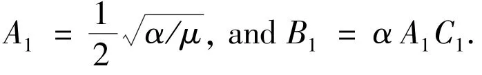
In Table 4,we present errors between exact and numerical solutions at different values of x and t in the region x∈[-10,10].The parameters are taken asΔx=0.01,Δt=0.01,andλ=c2/3.In comparison with ChSC(Chebyshev spectral collocation)method[30],results of the LBM are almost as good as numerical results obtained from Ref.[30].The traveling wave solutions obtained by the LBM,and the exact solutions of Eq.(27)are demonstrated in Fig.5 at time t=0.5.
Table 4 Absolute errors of LBM solutions at different values of x and t

Table 5 L∞and L2errors for various values ofα,β,andνat time t=0.5 and t=1 w ithμ=-0.1
Exam ple 6 Finally we consider Eqs.(1)and(5)with the following explicit traveling solitary wave solutions[2]

and

whereθ=x-vt+x0,v=-ν2/6μ-2μk2-α2/4β,and k=1,x0=0.
The L∞and L2errors for various values ofα,β,andνwithμ=-0.1 at time t=0.5 and t=1 are shown in Table5.In numerical simulation,the region of space is set in x∈[-10,10],and the parameters are taken asΔx=0.1,Δt=0.01,andλ=c2/2.Traveling solitary wave solutions obtained by LBM,and exact solutions of the cBKdV equation are displayed in Fig.6 at time t=5 withα=1,β=100,ν=0.01 andμ=-0.01.From the illustrations,we can see that the LBM results agree very wellwith the exact solutions.

Fig.5 LBM solutions and exact solutions at time t=0.5(traveling wave)

Fig.6 LBM solutions and exact solutions of cBKdV equation at t=5 withα=1,β=100,ν=0.01,andμ=-0.01
3 Conclusions
In this paper,a 3-bit lattice Boltzmannmodel for the cBKdV equation is proposed.By treating the dispersive term uxxxproperly and applying the Chapman-Enskog expansion,the governing equations are recovered correctly from the lattice Boltzmann equations and the local equilibrium distribution functions are also obtained.In order to illustrate efficiency of the proposed method, comparisons aremade with exact solutions and with other numerical results.Numerical experiments show that LBM results are not only in nice agreement with exact solutions but also much more accurate than those of othermethods.We shall discuss further works about thismodel in future.
[1] Wang M L.Exact solutions for a compound KdV-Burgers equation[J].Phys Lett A,1996,213:279-287.
[2] Feng Z S,Chen G.Solitary wave solutions of the compound Burgers Korteweg-de Vries equation[J].Physica A,2005,352:419-435.
[3] Pan X D.Solitary wave and similarity solutions of the combined KdV equation[J].Appl Math Mech, 1988,9:281-285.
[4] McIntosh I.Single phase averaging and traveling wave solutions of themodified Burgers-Korteweg-de Vries equation[J].Phys Lett A,1990,143:57-61.
[5] Canosa J,Gazdag J.The Korteweg-de Vries-Burgers equation[J].JComput Phys,1977,23:393-403.
[6] Johnson R S.A non-linear equation incorporating damping and dispersion[J].JFluid Mech,1970,42:49-60.
[7] Wijngaarden L V.One-dimensional flow of liquids containing small gas bubbles[J].Ann Rev Fluid Mech,1972,4:369-396.
[8] Gao G.A theory of interaction between dissipation and dispersion of turbulence[J].Sci Sin Ser A,1985, 28:616-627.
[9] Benzi R,Succi S,Vergassola M.The lattice Boltzmann equation:theory and applications[J].Phys Report,1992,222(3):145-197.
[10] Qian Y H,Succi S,Orszag S.Recent advances in lattice Boltzmann computing[J].Annu Rev Comput Phys,1995,3:195-242.
[11] Chen SY,Doolen G D.Lattice Boltzmannmethod for fluid flows[J].Annu Rev Fluid Mech,1998,30:329-364.
[12] Dawson SP,Chen SY,Doolen G D.Lattice Boltzmann computations for reaction-diffusion equations[J].JChem Phys,1993,2:1514-1523.
[13] Shen Z J,Yuan GW,Shen L J.Lattice Boltzmann method for Burgers equation[J].Chinese JComput Phys,2000,17:166-172.
[14] Yan GW.A lattice Boltzmann equation for waves[J].JComput Phys,2000,161:61-69.
[15] Yan GW,Zhang JY.A higher-odermomentmethod of the lattice Boltzmann model for the Korteweg-de Vries equation[J].Math Comput Simu,2009,79:1554-1565.
[16] Zhang JY,Yan GW.A lattice Boltzmannmodel for the Korteweg-de Vries equation with two conservation laws[J].Comput Phys Commu,2009,180:1054-1062.
[17] Duan Y L,Liu R X,Jiang Y Q.Lattice Boltzmann model for themodified Burgers’equation[J].Appl Math Comput,2008,202:489-497.
[18] Shi B C,Guo Z L.Lattice Boltzmann model for nonlinear convection-diffusion equations[J].Phy Rev E, 2009,79:016701.
[19] Shi B C,Deng B,Du R,Chen X W.A new scheme for source term in LBGK model for convectiondiffusion equation[J].Comput Math Appl,2008,55(7):1568-1575.
[20] Ma C F.A new lattice Blotzmannmodel for KdV-Burgers equation[J].Chinese Phys Lett,2005,22(9):2313-2315.
[21] Lai H L,Ma C F.Lattice Boltzmann method for the generalized Kuramoto-Sivashinsky equation[J].Physica A,2009,388:1405-1412.
[22] McNamara G R,Zanetti G.Use of the Boltzmann equation to simulate lattice-gas automata[J].Phys Rev Lett,1988,61:2332-2335.
[23] He X Y,Lou L S.Theory of the lattice Boltzmann method:from the Boltzmann equation to the lattice Boltzmann equation[J].Phy Rev E,1997,56:6811-6817.
[24] Bhatnagar P,Gross E,Krook M.A model for collision process in gas.I:Small amplitude processed in charged and neutral one component system[J].Phys Rev,1954,94:511-525.
[25] Guo Z L,Gross E,Krook M.Lattice Boltzmann method for Fluid Dynamics[M].Wuhan:Hubei Science and Technology Press,2002.
[26] Kutluay S,Bahadir A,Özdes A R.A small time solutions for the Korteweg-de Vries equation[J].Appl Math Comput,2000,107:203-210.
[27] Xiao M L,Wang R H,Zhu C G.Applyingmultiquadric quasi-interpolation to solve KdV equation[J].Journal of Mathematical Research Exposition,2011,31(2):191-201.
[28] Alexander M E,Morris J L I.Galerkin methods for some model equations for nonlinear dispersive wave [J].Comput Phys,1979,30:428-451.
[29] Soliman A A.Themodified extended tanh-functionmethod for solving Burgers-type equations[J].Physica A,2006,361:394-404.
[30] Khatera A H,Temsaha R S,Hassanb M M A.Chebyshev spectral collocationmethod for solving Burgers’-type equations[J].JComput Appl Math,2008,222:333-350.
Parallel Com puting of First-principles Based Quantum Transport Simulations
ZHANG Ruoxing1, HOU Shimin2, CHOU Qiang1
(1.National Energy Key Laboratory ofNuclear Power Software,Software Development Center,State Nuclear Power Technology Corporation,Beijing 100029,China;2.Key Laboratory for the Physics and Chemistry of Nanodevices,Department of Electronics,Peking University,Beijing 100871,China)
To solve long time-consuming problem in analysis of large-scale quantum transport systems based on first-principles calculations,we analyze hot spots of self-consistent iterations within the framework that combines non-equilibrium Green’s function with density functional theory,namely DFT+NEGFmethod.Two parallel computing schemes based on MPI/OpenMP are proposed to deal with energy point integration and matrix inversion/multiplication.For energy point integral parallelism,sparsematrix as well as energy points should be assigned to each process over data initialization according to round-robin scheduling algorithm.Either MPI based ScaLAPACK subroutine or OpenMP based Intel MKL subroutine can be called to realize matrix inversion/multiplication parallelization.A sub-linear speedup ratio curve is obtained for energy point integral parallelism due to the fact that calculations related with different energy points aremutually independent.OpenMP parallelism adopts shared memory patterned data exchangemechanism and overhead of switching threads is rather small,and consequently it is better in computing efficiency but worse in code scalability than MPI implementation.
first-principles calculations;density functional theory;Green’s function;MPI;parallel computing
Lattice Boltzmann M odel for Com pound Burgers-Korteweg-de Vries Equation
DUAN Yali1, CHEN Xianjin1, KONG Linghua2
(1.School ofMathematical Sciences,University of Science and Technology ofChina,Hefei,Anhui 230026,China;
2.School ofMathematicsand Information Science,Jiangxi Normal University,Nanchang,Jiangxi 330022,China)
1001-246X(2015)06-0639-10
O241.8 Document code:A
1001-246X(2015)06-0631-08
O411.2
A
2014-11-03;
2015-02-09
国家核电技术公司员工自主创新项目(SNP-KJ-CX-2015-27),大型先进压水堆核电站重大专项核电关键设计软件自主化技术研究课题(2011ZX06004-024)资助
张若兴(1980-),男,河北邢台,博士,高级工程师,主要研究领域为高性能网格计算和云计算、大数据分析技术、概率安全分析软件开发,E-mail:zhangruoxing@snptc.com.cn
Received date:2014-11-05;Revised date:2015-02-01
Foundation item s:Supported by the NSFC(11101399,10901074)and Fundamental Research Funds for Central Universities(WK0010000022)
Biography:Duan Yali(1973-),female,Shanxi,associate professor,Ph D,major in numerical solution of PDEs,E-mail:ylduan01@ustc.edu.cn
Abstract:We develop a lattice Boltzmannmodel for compound Burgers-Korteweg-de Vries(cBKdV)equation.By properly treating dispersive term uxxxand applying Chapman-Enskog expansion,the governing equation is recovered correctly from lattice Boltzmann equation and local equilibrium distribution functions are obtained.Numerical experiments show that our results agree well with exact solutions and have better numerical accuracy compared with previous numerical results.This hence indicates that the model is satisfactory and efficient.
Key words:Lattice Boltzmannmodel;Compound Burgers-KdV equation;Chapman-Enskog expansion
猜你喜欢
小学生学习指导·爆笑校园(2021年2期)2021-03-17
国防科技大学学报(2020年6期)2020-12-07
小读者(2020年4期)2020-06-16
测绘通报(2019年11期)2019-12-03
中国外汇(2019年20期)2019-11-25
赤峰学院学报·自然科学版(2019年5期)2019-09-10
电影(2018年12期)2018-12-23
测绘学报(2018年1期)2018-02-27
山东青年(2016年1期)2016-02-28
民主与科学(2014年3期)2014-02-28