北太平洋中层水模拟的改进❋
2016-11-10 03:25刘奇奇范植松胡瑞金刘海龙楚合涛
中国海洋大学学报(自然科学版) 2016年10期
刘奇奇, 范植松❋❋, 胡瑞金, 刘海龙, 楚合涛
(1.中国海洋大学海洋与大气学院,山东 青岛 266100; 2.中国科学院大气物理研究所,北京 100029; 3.莱西气象局,山东 莱西 266600)
北太平洋中层水模拟的改进❋
刘奇奇1, 范植松1❋❋, 胡瑞金1, 刘海龙2, 楚合涛3
(1.中国海洋大学海洋与大气学院,山东 青岛 266100; 2.中国科学院大气物理研究所,北京 100029; 3.莱西气象局,山东 莱西 266600)
通过对北太平洋中层水模拟和分析的3种结果的比较:在稀疏网格的LICOM全球大洋环流模式中使用Canuto等的湍流混合方案(简称T方案)并添加范植松等提出的惯性内波破碎混合方案(简称F方案),在LICOM模式中使用T方案,以及WOA09资料的分析结果,证明在添加F方案的情况下,北太平洋中层水的模拟有较明显的改进。惯性内波破碎混合可能是维持通风过程的重要机制之一,惯性频率风场的强迫作用可能是海洋内部混合的外部作用源。在WOA09资料的分析结果与数值模拟结果中均显示出北太平洋中层水的明显的季节变化,这意味着除表层水和模态水之外,北太平洋中层水在气候变化中扮演了重要的角色。模拟结果分析表明,为获得北太平洋中层水模拟的进一步改进,高分辨率的海洋模式和锋面与羽流的参数化方案是必要的。
垂直混合;惯性内波;通风过程;北太平洋中层水
引用格式:刘奇奇, 范植松, 胡瑞金, 等. 北太平洋中层水模拟的改进[J]. 中国海洋大学学报(自然科学版), 2016, 46(10): 1-9.
LIU Qi-Qi, FAN Zhi-Song, HU Rui-Jin, et al. An improvement of modeling the North Pacific intermediate water[J]. Periodical of Ocean University of China, 2016, 46(10): 1-9.
北太平洋中层水(North Pacific Intermediate Water,简称NPIW)的主要特征是具有整个水柱中盐度的最小值,其中心密度大约为1026.8kg/m3[1-2]。它在太平洋经向翻转环流中扮演着重要角色,其来源是Okhotsk海[3]和Alaska湾流[4]。Hasumi等曾提到“尽管北太平洋中层水非常重要,但对其模拟的研究却很少。粗网格模式对于模拟北太平洋中层水是不够的,因为其形成涉及了很多精细的过程,比如Okhotsk海水和北太平洋水的交换,Okhotsk海源头水的运输以及在混合水区域中的混合过程”[5]。Ishizaki和Ishikawa曾用过高分辨率模式来模拟北太平洋中层水[6],并进行改进[7]。除了上述Hasumi等人指出的精细过程,作者认为海洋内部的垂直混合(跨等密度面混合)过程的参数化是模拟北太平洋经向翻转环流的关键,也是模拟北太平洋中层水的关键。众所周知,海洋内部的垂直混合过程和风生南大洋Ekman上升流驱动了全球的经向翻转环流[8-10]。然而,不同于北大西洋,在北太平洋,风生南大洋Ekman上升流对经向翻转环流影响很小。

在F方案中考虑了惯性内波破碎产生的细结构的扰动引起的垂直效应[13-14]。使用Canuto等的湍流混合方案(简称为T方案)[29],并添加F方案,对全球海洋的温度和盐度的模拟获得显著的改进,特别是在中高纬度区域的中层水和深层水的模拟。如文献[13]中图7~10所示,相对于初始场(WOA05资料)对太平洋的中层水和深层水模拟的盐度和温度的年平均相对误差和均方差根误差的统计结果显示明显的改进。依据这些模拟结果,本文进行模拟北太平洋中层水的比较研究。
1 研究基础
1.1 LICOM模式
LICOM是中国科学院大气物理研究所(IAP)大气科学和地球流体力学数值模拟国家重点实验室(LASG)开发的全球海洋环流模式(OGCM)[30]。它的水平分辨率是1(°)×1(°),垂直分为30层(300m深度之上为12层)。目前LICOM模式采用的混合方案是T方案,将在1.2节中介绍。依据该模式进行了气候平均态全球大洋数值试验。模拟时间为200年,初始无运动温度与盐度场为WOA05资料。在本次试验中,采用了2种不同混合方案:单独使用T方案和T方案添加F方案,F方案在1.3节中给出。模式在运行到151a时达到基本稳定。主要考虑盐度、温度和其它参数在151~200a的平均值。
1.2 湍流混合方案(T方案)
通过改进Mellor和Yamada模式,Canuto等提出OGCM中比较新的湍流混合方案(T方案)[29,31-32]。T方案最显著的改进是将Mellor和Yamada模式的临界Richardson数由Ricr=0.2改为Ricr~1。另外,在该新方案中考虑了盐指的发生。
1.3 惯性内波破碎混合方案(F方案)
不同于湍流混合方案,F方案中考虑了由细尺度近惯性内波(可逆细结构)所产生斑块的垂直徙动。所使用的内波能量谱E(β,θ,ω)为[13]:
(1)

(2)

(3)

(4)

(5)
A(β)=
(6)

(7)
细结构的水平动能谱Hsf(ω)为:

(8)
近惯性频段的水平动能谱Ek为:

(9)
细结构的位移谱Dsf(ω)为:

(10)
近惯性频段的势能Ep为:
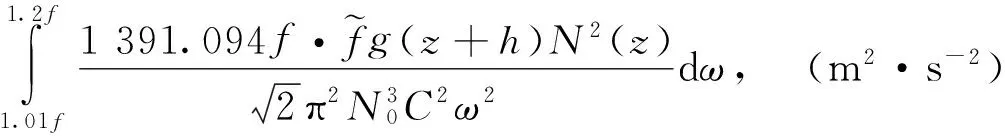
(11)
细结构的剪切谱Φsf(β,ω)为:
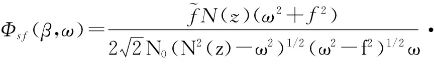

(12)
由惯性内波破碎混合产生的动量的垂直涡旋粘性系数Av和温度/盐度垂直涡旋扩散系数Kv分别由以下两个公式计算:

(13)
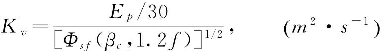
(14)
这里:

(15)
βc=0.1cpm=0.1×2π,(rad/m)。
(16)
h=4500m;N0=5.235988×10⁻³rad/s;b=1300m;π=3.14159;g=9.8m/s2;C=1500m/s。
(17)
因为在主温跃层中,相对于等盐度面,等位势密度面更接近于等温度面,所以沿等位势密度面产生的破碎产物中温度的分布比起盐度来更为均匀。因此,对应于斑块垂直徙动的温度的垂直涡旋扩散系数比盐度的相应值更小。本文假定在主温跃层中的温度的垂直涡旋扩散系数Kt为:
Kt=Ks/5 。
(18)
这里的Ks是深度小于1500m的水层中盐度垂直扩散系数Kv,计算公式为(14)式。本模式的坐标原点(z=0)设立在混合层底部。公式(18)是F方案独有的,与湍流混合方案不同。通常在OGCM中只考虑湍流混合,并采用盐度扩散系数与温度扩散系数一致。例如,Nash和Moum依据海洋测量结果获得如下的关系[33]:
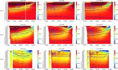
dt=Kts/Ktt,0.6 (19) 这里dt是海洋中湍流混合盐度扩散系数Kts和温度扩散系数Ktt的比例。而在层化栅格湍流的室内实验中,Rehmann和Koseff的结果为[34]: 0.67 (20) 但误差范围较大。 在赤道海洋(15°S~15°N),由于强剪切的背景流和内波的水平各向异性[35-36],内波能量谱E(β,θ,ω)的计算公式(1)~(7)不适用。另外,考虑到风生惯性内波主要在中高纬度海域盛行[16,28],本文建议在(15°S~15°N)之外的区域将F方案添加到T方案,在赤道区域仅用T方案。 2.1 北太平洋中层水的垂直剖面结构 本文中选取北太平洋中层水团中密度值为1026.8kg/m3的等密度面附近的水柱中盐度最小值曲面作为该水团的中心表示。为了揭示F方案对模拟北太平洋中层水及对其形成和传输机制理解的优势,本文中采用了2个方法,即北太平洋中层水的垂直剖面结构的比较研究和其水平分布形态的比较研究,并分别以1月的模拟结果代表冬季,7月模拟结果代表夏季。 图1为北太平洋中层水的垂直剖面结构的比较,分别为在稀疏网格的LICOM模式中使用T方案添加F方案(表示为“LICOM+F”),在LICOM模式中仅使用T方案(表示为“LICOM”),以及WOA09资料的分析结果(表示为“WOA09”)。对应剖面的经度分别为150°E,180°E和210°E,使用1月份1500m以上深度的数据。图2与图1类似,为沿20°N,30°N和40°N的1月份纬度剖面结构的比较。图1和2清楚地显示使用F方案显著改善了对北太平洋中层水的模拟,而且盐度模拟的改进更为明显。该成果意味着使用F方案能更好的模拟通风过程。如图1~6所示,从Okhotsk海和Alaska湾流流入的低温低盐水向下俯冲混合并且在低纬度地区向上涌升,俯冲的最深深度能达到1000m左右。源头水通过副极地环流圈、混合水区域的混合过程以及副热带环流圈在北太平洋散布开来。在这个通风过程中不能仅考虑湍流混合(T方案),也应考虑惯性内波破碎混合(F方案)。而且在F方案中盐度垂直涡旋扩散系数Ks的特殊性质(公式(18))是适宜的。 稀疏网格LICOM模式的局限性在图1中150°E剖面的高纬度地区清晰地显示出来,而且在图5中Okhotsk海及其邻近西北太平洋区域也显示出来。在这些区域,模拟结果相当不同于观测结果(WOA09),甚至没有合理的值。引起该缺陷的原因有2个:粗网格分辨率和海冰模式。在1月份(冬季),Okhotsk海以及西北太平洋附近有大量的海冰存在,然而粗网格分辨率LICOM模式和海冰模式不能适当地模拟出该区域的海况,以及Okhotsk海和北太平洋的海水交换。另外,图2中40°N剖面图中的日本海宽度清楚地小于真实情况,这也将会影响日本海和西北太平洋的模拟结果。 (在稀疏网格的LICOM模式中使用T方案添加F方案(表示为“LICOM+F”),在LICOM模式中仅使用T方案(表示为“LICOM”),以及WOA09资料的分析结果(表示为“WOA09”)。对应剖面的经度分别为150°E,180°E和210°E,使用1月份1500m以上深度的数据。图中彩色背景为盐度(psu);黑色实线为等温线(℃);蓝色点线是等位密度线(kg/m3);白色虚线是混合层底部深度(m);红色实线是选取的NPIW中心表示;横坐标是北半球纬度;纵坐标为水深(m)。Depicted are the results simulated by performing the coarse-resolution LICOM with T-scheme adding F-scheme (denotation “LICOM+F”), those simulated with T-scheme alone (denotation “LICOM”), and the WOA09 data (denotation “WOA09”), against latitude along longitude 150°E, 180°E and 210°E respectively, in January above the depth of 1500m. In each panel, salinity is denoted with background color (psu); Black solid curve represents isotherm (℃); Blue dotted curve represents potential isopycnal (kg/m3); White dotted curve represents the mixed layer base (m); Red solid curve is the centre representation of NPIW; Abscissa is latitude in the north hemisphere, and ordinate is the depth of water (m).) 图1北太平洋中层水的经度垂直剖面结构的比较 Fig.1Comparison among simulation results of vertical profile structure along longitude of NPIW (与图1相似,但是分别为20°N,30°N和40°N的纬度剖面结构的比较。As in Fig.1, but against longitude along latitude 20°N, 30°N and 40°N respectively.) 图2 北太平洋中层水的纬度垂直剖面结构的比较Fig.2 Comparison among simulation results of vertical profile structure along latitude of NPIW (与图1相似,但是为7月份。As in Fig.1, but in July.) 图3 北太平洋中层水的经度垂直剖面结构的比较Fig.3 Comparison among simulation results of vertical profile structure along longitude of NPIW (与图2相似,但是为7月份。As in Fig.2, but in July.) 图4 北太平洋中层水的纬度垂直剖面结构的比较Fig.4 Comparison among simulation results of vertical profile structure along latitude of NPIW (在稀疏网格的LICOM模式中使用T方案添加F方案(表示为“LICOM+F”),在LICOM模式中仅使用T方案(表示为“LICOM”),以及WOA09资料的分析结果(表示为“WOA09”)。对应的盐度(psu)、温度(℃)和中心表示层深度(m)的水平分布图所依据的数据均为1月份数据。Depicted are the simulation results of horizontal distribution pattern of salinity (psu), temperature (℃) and the depth (m) of the centre representation of NPIW by performing the coarse-resolution LICOM with T-scheme adding F-scheme (denotation “LICOM+F”), those simulated with T-scheme alone (denotation “LICOM”), and the WOA09 data (denotation “WOA09”) respectively in January.) 图5北太平洋中层水的水平分布形态的比较 Fig.5Comparison among simulation results of horizontal distribution pattern of NPIW (与图5相似,但是为7月份。As in Fig.5, but in July.) 图6 北太平洋中层水的水平分布形态的比较Fig.6 Comparison among simulation results of horizontal distribution pattern of NPIW 与图1和2类似,7月份的模拟结果示于图3和4。北太平洋中层水的主要特性以及F方案的优势从1月维持到了7月,但从图1~4中可观察到NPIW明显的季节变化。观测资料(WOA09)和模拟结果都呈现出季节变化,这是因为来自Okhotsk海和Alaska湾流的源头水具有强烈的季节变化特性。该季节变化暗示除了表层水和模态水,NPIW在气候变化中扮演重要的角色[5]。NPIW对气候变化的响应及其在北太平洋长期变化中的作用是有待研究的重要课题。 2.2 北太平洋中层水的水平分布形态 另一个研究方法是北太平洋中层水的水平分布形态的比较研究。图5给出了1月(冬季)北太平洋中层水的水平分布形态的比较,分别为在稀疏网格的LICOM模式中使用T方案添加F方案(表示为“LICOM+F”),在LICOM模式中仅使用T方案(表示为“LICOM”),以及WOA09资料的分析结果(表示为“WOA09”)。对应的盐度(psu)、温度(℃)和中心表示层深度(m)的水平分布图所依据的数据均为1月份在中心表示曲面上的数据。图6与5相似,是7月(夏季)的比较结果。与上述的NPIW垂直剖面结构比较相似,使用F方案在NPIW的盐度、温度、中心表示层深度的水平分布模拟方面的改进是明显的。另外,在图5和6中NPIW的季节变化也清楚地显示出来。 值得注意的是,在图5中Okhotsk海和西北太平洋附近的模拟结果中存在明显的空白区域,此与图1中150°E剖面图中高纬度区域相对应,这是由2.1节中提到的不足之处所引起。 通过以上的比较研究可得出结论如下: (1)在稀疏网格的LICOM全球大洋环流模式中使用湍流混合方案(T方案)添加惯性内波破碎混合方案(F方案),模拟北太平洋中层水的成果表明F方案是强有效的。 (2)为获得北太平洋中层水模拟的进一步改进,高分辨率的海洋模式和锋面与羽流的参数化方案是必要的。 [1]Talley L D. An Okhotsk Sea water anomaly: implications for ventilation in the North Pacific [J]. Deep-Sea Res, 1991, 38: S171-S190. [2]Talley L D. Distribution and formation of North Pacific intermediate water [J]. J Phys Oceanogr, 1993, 13: 517-537. [3]Yasuda I. The origin of the North Pacific intermediate water [J]. J Geophys Res, 1997, 102: 893-909. [4]You Y, Suginohara N, Fukasawa M, et al. Roles of the Okhotsk Sea and Gulf of Alaska in forming the North Pacific intermediate water [J]. J Geophys Res, 2000, 105: 3253-3280. [5]Hasumi H, Tatebe H, Kawasaki T, et al. Progress of North Pacific modeling over the past decade [J]. Deep-Sea Res II, 2010, 57: 1188-1200. doi: 10. 1016/j. dsr2. 2009. 12. 008. [6]Ishizaki H, Ishikawa I. Simulation of formation and spreading of salinity minimum associated with NPIW using a high-resolution model [J]. J Oceanogr, 2004, 60: 463-485. [7]Ishikawa I, Ishizaki H. Importance of eddy representation for modeling of the intermediate salinity minimum in the North Pacific in comparison between eddy-resolving and eddy-permitting models [J]. J Oceanogr, 2009, 65: 407-426. [8]Munk W, Wunsch C. Abyssal recipes II: Energetics of tidal and wind mixing [J]. Deep Sea Res Part I, 1998, 45(12): 1977-2010. [9]Wunsch C, Ferrari R. Vertical mixing, energy and the general circulation of the oceans [J]. Annu Rev Fluid Mech, 2004, 36(1): 281-314. [10]Kuhlbrodt T, Griesel A, Montoya M, et al. On the driving processes of the Atlantic meridional overturning circulation [J]. Rev Geophys, 2007, 45: RG2001, doi: 10. 1029/2004RG000166. [11]Nasmyth P. Oceanic Turbulence [D]. Vancouver, Canada: Institute of Oceanography, University of British Columbia, 1970. [12]Oakey N S. Determination of the rate of dissipation of turbulent energy from simultaneous temperature and velocity shear microstructure measurements [J]. J Phys Oceanogr, 1982, 12(3): 256-271. [13]Fan Z S, Shang Z Q, Zhang S W, et al. A parameterization scheme of vertical mixing due to inertial internal wave breaking in the ocean general circulation model [J]. Acta Oceanol Sin, 2015, 34(1): 11-22. doi: 10. 1007/s13131-015-0591-1. [14]尚真琦, 刘海龙, 范植松, 等. LICOM模式中不同混合方案的比较研究 [J]. 中国海洋大学学报(自然科学版), 2015, 45(10): 1-6. doi: 10. 16441/j. cnki. hdxb. 20140288. Shang Z Q, Liu H L, Fan Z S, et al. A comparative study of different mixing schemes in framework of the LICOM (in Chinese)[J]. Periodical of Ocean University of China, 2015, 45(10): 1-6. doi: 10. 16441/j. cnki. hdxb. 20140288. [15]Müller P, Olbers D, Willebrand J. The IWEX spectrum [J]. J Geophys Res, 1978, 83(C1): 479-500. [16]Gregg M C, D’Asaro E A, Shay T J, et al. Observations of persistent mixing and near-inertial internal waves [J]. J Phys Oceanogr, 1986, 16(5): 856-885. [17]Kunze E, Briscoe M G, Williams III A J. Interpreting shear and strain fine structure from a neutrally buoyant float [J]. J Geophys Res, 1990, 95(C10): 18111-18125. [18]Kunze E, Williams III A J, Briscoe M G. Observations of shear and vertical stability from a neutrally buoyant float [J]. J Geophys Res, 1990, 95(C10): 18127-18142. [19]Pinkel R, Sherman J, Smith J, et al. Strain: observations of the vertical gradient of isopycnal vertical displacement [J]. J Phys Oceanogr, 1991, 21: 527-540. [20]Shcherbina A Y, Sundermeyer M A, Kunze E, et al. The LatMix summer campaign: submesoscale stirring in the upper ocean [J]. Bulletin of the American Meteorological Society, 2014. doi: 10. 1175/BAMS-D-14-00015. 1. [21]范植松, 方欣华. 旋转向量水平分量对大洋内波方程的影响[J]. 海洋学报, 1998, 20(3): 129-133. Fan Z S, Fang X H. Effect of horizontal component of rotation vector on equations for oceanic internal waves[J]. Acta Oceanologica Sinica (in Chinese), 1998, 20(3): 129-133. [22]范植松, 方欣华. 考虑旋转向量水平分量的大洋内波方程的一个渐近解 [J]. 海洋学报, 1998, 20(4): 1-8. Fan Z S, Fang X H. An asymptotic solution of equations for oceanic internal waves under considering horizontal component of rotation vector[J]. Acta Oceanologica Sinica (in Chinese), 1998, 20(4): 1-8. [23]Fan Z S, Fang X H. A possible mechanism of ocean finestructure. Part I: Energy and coherence [J]. Journal of Ocean University of Qingdao, 1999, 29(2): 207-214. [24]Fan Z S, Fang X H, Xu Q C. A possible mechanism of ocean finestructure. Part II: Shear and strain [J]. Journal of Ocean University of Qingdao, 1999, 29(3): 405-414. [25]Fan Z S, Fang X H. A possible mechanism of ocean finestructure. Part III: Estimation of the kinetic energy dissipation in mixing [J]. Journal of Ocean University of Qingdao, 2000, 30(1): 7-14. [26]Fan Z S. Is the small-scale turbulence an exclusive breaking product of oceanic internal waves [J]. Acta Oceanol Sin, 2011, 30(6): 1-11. [27]Garrett C J R. What is the “near-inertial” band and why is it different from the rest of the internal wave spectrum? [J]. J Phys Oceanogr, 2001, 31: 962-971. [28]Alford M H, Cronin M F, Klymak J M. Annual cycle and depth penetration of wind-generated near-inertial internal waves at Ocean Station Papa in the Northeast Pacific [J]. J Phys Oceanogr, 2012, 42(6): 889-909. doi: 10. 1175/JPO-D-11-092. 1. [29]Canuto V M, Howard A, Cheng Y, et al. Ocean turbulence, III: new GISS vertical mixing scheme [J]. Ocean Modelling, 2010, 34(3-4): 70-91. doi: 10. 1016/j. ocemod. 2010. 04. 006. [30]刘海龙, 俞永强, 李薇, 等. LASG/LAP 气候系统海洋模式(LICOM1. 0)参考手册[M]. 北京: 科学出版社, 2004: 107. Liu H, Yu Y, Li W, and Zhang X. 2004. Reference Manual for LASG/IAP Climate System Ocean Model (LICOM1. 0). Beijing: Science Press, China, 2004, 107 (in Chinese). [31]Canuto V M, Howard A, Cheng Y, et al. Ocean turbulence. Part I: one point closure model, momentum and heat vertical diffusivities [J]. J Phys Oceanogr, 2001, 31(6): 1413-1426. [32]Canuto V M, Howard A, Cheng Y, et al. Ocean turbulence. Part II: vertical diffusivities of momentum, heat, salt, mass and passive scalars[J]. J Phys Oceanogr, 2002, 32: 240-264. [33]Nash J D, Moum J N. Microstructure estimates of turbulent salinity flux and the dissipation spectrum of salinity [J]. J Phys Oceanogr, 2002, 32: 2312-2333. [34]Rehmann C R, Koseff J R. Mean potential energy change in stratified grid turbulence [J]. Dynamics of Atmospheres and Oceans, 2004, 37: 271-294. [35]Eriksen C C. Some characteristics of internal gravity waves in the equatorial Pacific [J]. J Geophys Res, 1985, 90(C4): 7243-7255. [36]Boyd T J, Luther D S, Knox R A, et al. High-frequency internal waves in the strongly sheared currents of the upper equatorial Pacific: Observations and a simple spectral model [J]. J Geophys Res, 1993, 98(C10): 18089-18107. [37]Hibiya T, Nagasawa M, Niwa Y. Global mapping of diapycnal diffusivity in the deep ocean based on the results of expendable current profiler (XCP) surveys [J]. Geophys Res Lett, 2006, 33: L03611. doi: 10. 1029/2005GL025218. 责任编辑庞旻 An Improvement of Modeling the North Pacific Intermediate Water LIU Qi-Qi1, FAN Zhi-Song1, HU Rui-Jin1, LIU Hai-Long2, CHU He-Tao3 (1.College of Oceanic and Atmospheric Sciences, Ocean University of China, Qingdao 266100, China; 2.State Key Laboratory of Numerical Modeling for Atmospheric Sciences and Geophysical Fluid Dynamics, Institute of Atmospheric Physics, Chinese Academy of Sciences, Beijing 100029, China; 3.Laixi Meteorological Bureau, Laixi 266600, China) The comparison among results simulated by performing the coarse-resolution LICOM model over the global ocean with the turbulence mixing scheme of Canuto et al. (T-scheme for short) adding the inertial internal wave breaking mixing scheme (F-scheme for short) put forward by Fan et al. recently, those simulated with T-scheme alone, and the WOA09 data, demonstrates that a notable improvement of modeling the North Pacific Intermediate Water (NPIW) has been attained by using F-scheme, which illustrates the robustness and effectiveness of F-scheme. The inertial internal wave breaking mixing may be one of important mechanisms maintaining the ventilation process, as well as inertial forcing of wind may be an external mechanical source of mixing in the ocean interior. The obvious seasonal variability of NPIW occurs in both the observations (WOA09) and the simulation results, which implies that NPIW plays an important role in climate changes besides the surface water and Mode water. Finally analysis of the simulation results indicates that to achieve further progress of modeling NPIW the high-resolution ocean model and the parameterization scheme of fronts and filaments are necessary. vertical mixing; inertial internal wave; ventilation process; North Pacific intermediate water 国家自然科学基金面上项目(41275084)资助 2016-03-07; 2016-04-24 刘奇奇(1990-),女,硕士生。E-mail: lqqi1990@163.com ❋❋通讯作者:E-mail:fanzhs@hotmail.com P722 A 1672-5174(2016)10-001-09 10.16441/j.cnki.hdxb.20160056 Supported by the National Natural Science Foundation of China(41275084)2 数值模拟


3 结论与讨论
猜你喜欢
传染病信息(2022年6期)2023-01-12海洋通报(2022年6期)2023-01-07土木工程与管理学报(2021年6期)2022-01-12电脑报(2021年20期)2021-08-10空间科学学报(2021年2期)2021-07-21海洋学报(2020年9期)2020-10-09空间科学学报(2020年2期)2020-04-01航空材料学报(2017年1期)2017-02-17肿瘤影像学(2015年3期)2015-12-09现代企业(2015年6期)2015-02-28