New Exact Traveling Wave Solutions of the Unstable Nonlinear Schrodinger Equations

K.HosseiniD.KumarM.Kaplanand E.Yazdani Bejarbaneh

1Department of Mathematics,Rasht Branch,Islamic Azad University,Rasht,Iran

2Graduate School of Systems and Information Engineering,University of Tsukuba,Tennodai 1-1-1,Tsukuba,Ibaraki,Japan

3Department of Mathematics,Bangabandhu Sheikh Mujibur Rahman Science and Technology University,Gopalganj-8100,Bangladesh

4Department of Mathematics,Art-Science Faculty,Kastamonu University,Kastamonu,Turkey

5Young Researchers and Elite Club,Qazvin Branch,Islamic Azad University,Qazvin,Iran

1 Introduction

Generally,the nonlinear Schrodinger equation(NLSE)[1]

In the past several years,various powerful methods[6−19]have been developed and also employed to look for the exact solutions of nonlinear differential equations.Recently,Luet al.[20]executed the extended form of simple equation method to find some exact solutions of the unstable nonlinear Schrodinger equation(UNLSE)and the modi fied unstable nonlinear Schrodinger equation(modi fied UNLSE)which are expressed by Eqs.(2)and(3)as

whereλandγare real constants.If we considerγ=0,then Eqs.(2)and(3)are reduced to the NLSE(1).The main aim of this study is to produce new exact traveling wave solutions of the UNLSE and its modi fied form using two efficient distinct methods,known as the modified Kudryashov method and the sine-Gordon expansion approach.

The rest of this paper is arranged as follows:Sections 2 and 3 indicate how to adopt the modi fied Kudryashov method and the sine-Gordon expansion approach for acquiring new exact traveling wave solutions of the unstable nonlinear Schrodinger equation and its modi fied form.Finally,Sec.4 provides a conclusion remark about the results generated.

2 Modi fied Kudryashov Method for Solving the Unstable Nonlinear Schrodinger Equations

The modi fied Kudryashov method[21−25]is considered as a new problem-solving technique that has received considerable attention to find new exact solutions of nonlinear differential equations used in mathematical physics.First,we present a brief description about the modi fied Kudryashov method to obtain new exact solutions for a given nonlinear partial differential equation.For this goal,consider a nonlinear partial differential equation as

where the functionu=u(x,t)is unknown andFis a polynomial.The main steps are as follows:

Step 1Introducing the transformationu(x,t)=U(ξ)whereξ=kx+ωt,varies Eq.(4)to the following nonlinear ordinary differential equation

whereGis a polynomial ofUand its derivatives such that the superscripts indicate the ordinary derivatives with respect toξ.

Step 2Let us assume that the solutionU(ξ)of the nonlinear Eq.(5)can be presented as

in which the constantsai(i=0,1,...,N)are determined latter,Nis a positive integer which can be computed by means of balance principle,andQ(ξ)satis fies the following new equation

with the exact solutionQ(ξ)=1/(1+daξ).

Step 3By substituting Eq.(6)along with Eq.(7)into Eq.(5)and using some mathematical operations,we get a system of algebraic equations.

Step 4Solving the generated system and setting the obtained values in Eq.(6), finally produces new exact solutions for Eq.(4).

2.1 Solutions of the Unstable Nonlinear Schrodinger Equation

By considering the following transformation

the unstable nonlinear Schrodinger equation(2)can be reduced to a nonlinear ordinary differential equation as below

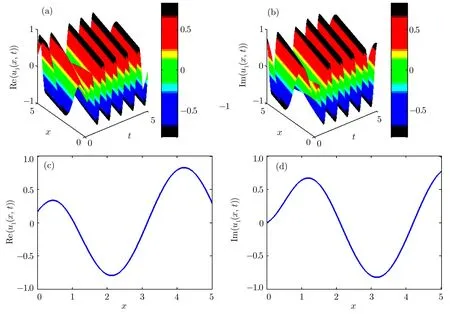
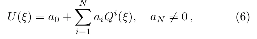
Fig.1 (a)–(b)3D graphs of the solution of unstable Schrodinger equation obtained by the modi fied Kudryashov method for the parameters a=3,k=1.5,p=1.5,d=1.5,and γ =1.5.(c)–(d)2D graphs of(a)–(b)at t=0.

Using the homogeneous balance principle,we findN=1.Then,the solution of Eq.(8)takes the form

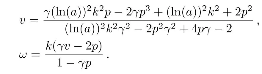
By substituting Eq.(9)along with its second order derivative into Eq.(8)and comparing the terms in the resulting equation,a nonlinear system is gained which by solving it,we find

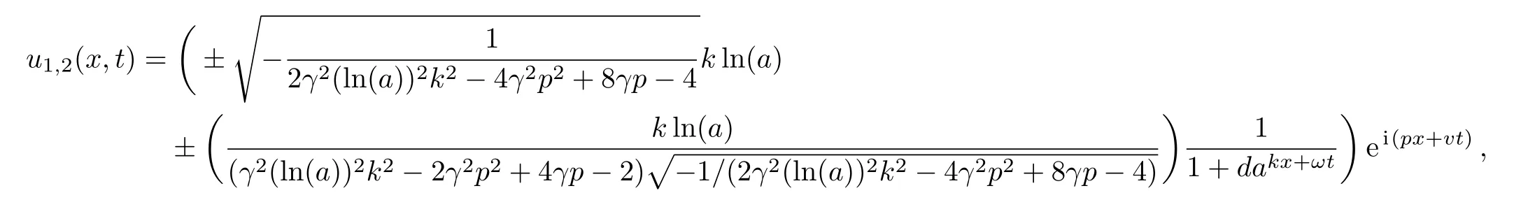
Now,the following new exact traveling wave solutions to the UNLSE are extracted

3D and 2D graphs ofu1(x,t)of the unstable nonlinear Schrodinger equation obtained by the modi fied Kudryashov method have been demonstrated in Fig.1.

2.2 Solutions of the Modi fied Unstable Nonlinear Schrodinger Equation

By introducing the following transformation

the modi fied unstable nonlinear Schrodinger equation(3)can be converted to a nonlinear ordinary differential equation as follows

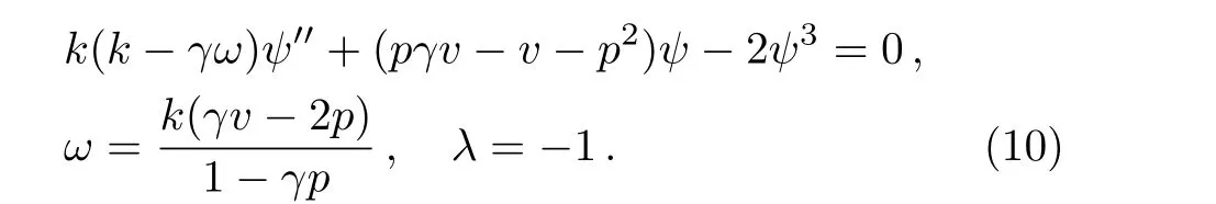
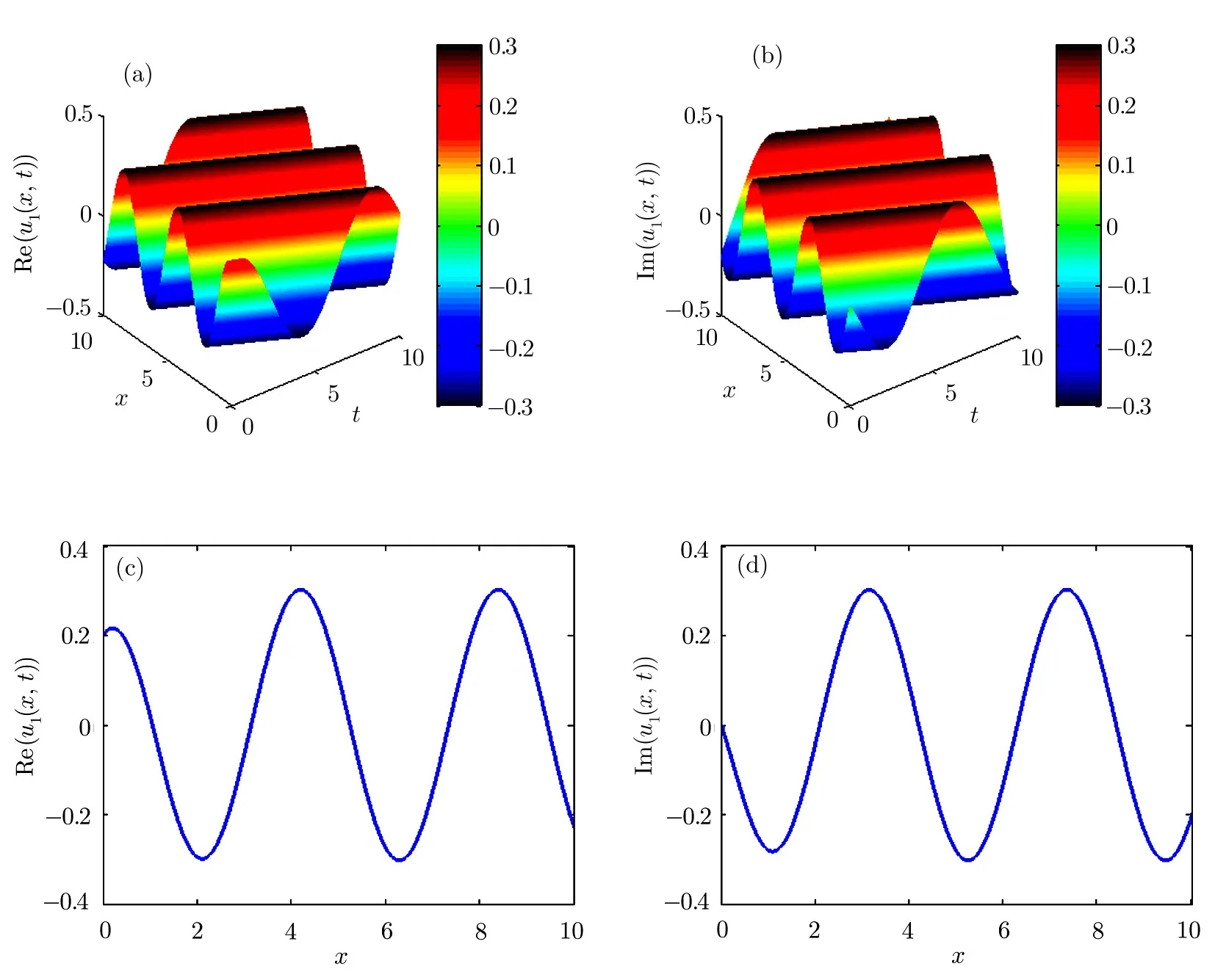
Fig.2 (a)–(b)3D graphs of the solution of modi fied unstable Schrodinger equation obtained by the modi fied Kudryashov method for the parameters a=3,k=1.5,p= −1.5,d=5,and γ =1.5.(c)–(d)2D graphs of(a)–(b)at t=0.

Using the homogeneous balance principle,we obtainN=1.Then,the solution of Eq.(10)can be written

By setting Eq.(11)along with its second order derivative in Eq.(10)and comparing the terms in the resulting equation,a nonlinear system is acquired which by solving it,we obtain

Now,the following new exact solutions to the modi fied UNLSE are generated

in which

3D and 2D graphs ofu1(x,t)of the modi fied unstable nonlinear Schrodinger equation derived by the modi fied Kudryashov method have been shown in Fig.2.

3 Sine-Gordon Expansion Approach for Solving the Unstable Nonlinear Schrodinger Equations

The sine-Gordon expansion method[26−29]is one of the most efficient techniques for seeking the exact solutions of various forms of nonlinear differential equations.The fundamental of the sine-Gordon expansion approach can be summarized as follows.

Consider the sine-Gordon equation which is presented as

Considering the transformationu(x,t)=U(ξ)whereξ=kx+ωt,converts Eq.(12)to a nonlinear ordinary differential equation as

MultiplyingU′on the both sides of Eq.(13)and integrating it once yields

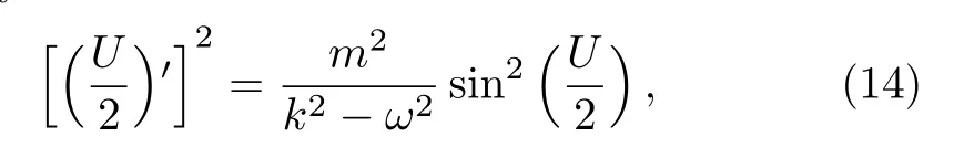
where the integration constant is taken to be zero.

By insertingU/2=w(ξ)andm2/(k2−ω2)=a2in Eq.(14),we find

For convenience,we considera=1 in Eq.(15),and so

The nontrivial solutions of Eq.(16)are as follows

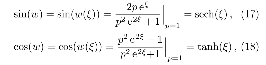
wherep/=0 is the integration constant.

Now,consider the following nonlinear partial differential equation

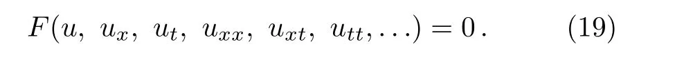
Introducing the transformationu(x,t)=U(ξ)whereξ=kx+ωt,reduces Eq.(19)to a nonlinear ordinary differential equation as

Suppose that the solution of Eq.(20)can be expressed as

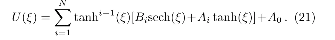
Now,using Eqs.(17)and(18),Eq.(21)can be rewritten as the following form

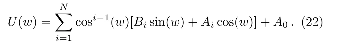
Calculating the positive integerNusing the homogeneous balance technique,setting Eq.(22)in Eq.(20),and comparing the terms,yields a nonlinear algebraic system which by solving it;we get the exact traveling wave solutions of Eq.(19).

3.1 Solutions of the Unstable Nonlinear Schrodinger Equation

From previous section,we haveN=1.As a result,Eq.(8)has a finite series solution in the form

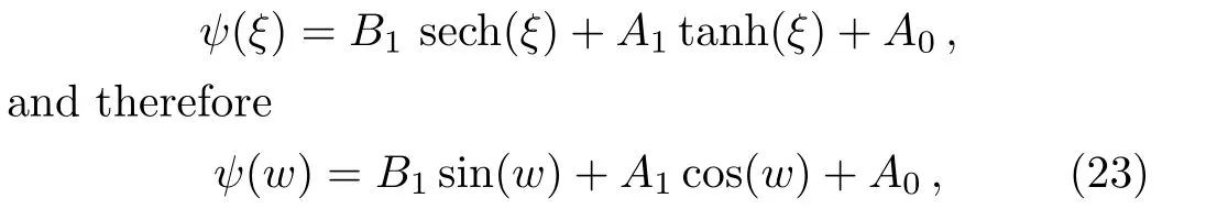
where eitherA1orB1may be zero,but bothA1orB1cannot be zero simultaneously.

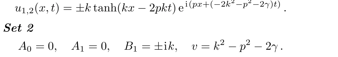
By inserting Eq.(23)in Eq.(8)and comparing the terms,we obtain a nonlinear algebraic system whose solution yields:

Now,the following exact traveling wave solutions to the UNLSE are extracted

Now,the following exact traveling wave solutions to the UNLSE are generated

Now,the following exact traveling wave solutions to the UNLSE are produced

Now,the following exact traveling wave solutions to the UNLSE are generated

3D and 2D graphs ofu5(x,t)of the unstable nonlinear Schrodinger equation obtained by the sine-Gordon expansion approach have been illustrated in Fig.3.

Fig.3 (a)–(b)3D graphs of the solution of unstable Schrodinger equation obtained by the sine-Gordon expansion approach for the parameters k=1.5,p=1.5,and γ =1.5.(c)–(d)2D graphs of(a)–(b)at t=0.

3.2 Solutions of the Modi fied Unstable Nonlinear Schrodinger Equation

As before,we haveN=1.As a consequence,Eq.(10)has a finite series solution as below

where eitherA1orB1may be zero,but bothA1orB1cannot be zero simultaneously.

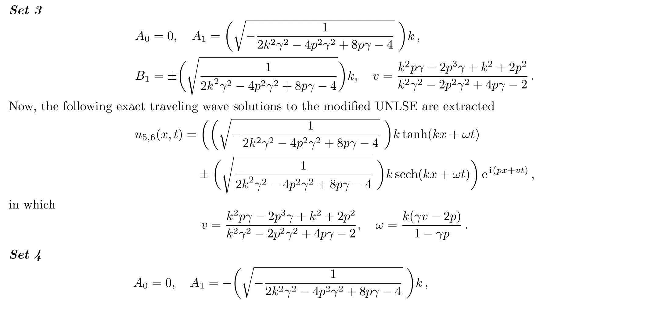
By setting Eq.(24)in Eq.(10)and comparing the terms,we acquire a nonlinear algebraic system whose solution results in:

Now,the following exact traveling wave solutions to the modi fied UNLSE are generated

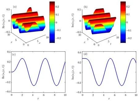
Fig.4 (a)–(b)3D graphs of the solution of modi fied unstable Schrodinger equation obtained by the sine-Gordon expansion approach for the parameters k=1.5,p= −1.5,and γ =1.5.(c)–(d)2D graphs of(a)–(b)at t=0.

3D and 2D graphs ofu7(x,t)of the modi fied unstable nonlinear Schrodinger equation derived by the sine-Gordon expansion approach have been demonstrated in Fig.4.

4 Conclusion

The unstable nonlinear Schrodinger equations,describing the time evolution of disturbances in marginally stable or unstable media were studied,successfully.The modi fied Kudraysov method and the sine-Gordon expansion approach were used as two new effective techniques to solve the unstable nonlinear Schrodinger equation and its modi fied form.As an outcome,a number of new exact traveling wave solutions for the unstable nonlinear Schrodinger equation and its modi fied form were formally derived.It should be stated the credibility of the results reported in this paper was examined by putting each new solution back into its corresponding equation.

[1]A.Ebaid and S.M.Khaled,J.Comput.Appl.Math.235(2011)1984.

[2]N.Taghizadeh,M.Mirzazadeh,and F.Farahrooz,J.Math.Anal.Appl.374(2011)549.

[3]S.M.Rayhanul Islam,World Appl.Sci.J.33(2015)659.

[4]M.G.Hafez,Beni-Suef Univ.J.Basic Appl.Sci.5(2016)109.

[5]M.Kaplan,o.¨Unsal,and A.Bekir,Math.Methods Appl.Sci.39(2016)2093.

[6]A.R.Seadawy,J.Electromagn.Waves Appl.(2017),doi:10.1080/09205071.2017.1348262.

[7]M.Inc,Optik 138(2017)1.

[8]M.Mirzazadeh,M.Ekici,Q.Zhou,and A.Sonmezoglu,Superlattices Microstruct.101(2017)493.

[9]N.Taghizadeh,Q.Zhou,M.Ekici,and M.Mirzazadeh,Superlattices Microstruct.102(2017)323.

[10]M.Naja fiand S.Arbabi,Commun.Theor.Phys.62(2014)301.

[11]E.M.E.Zayed and Y.A.Amer,Comput.Math.Modeling 28(2017)118.

[12]M.Ekici,Q.Zhou,A.Sonmezoglu,et al.,Superlattices Microstruct.107(2017)197.

[13]M.Younis,Mod.Phys.Lett.B 31(2017)1750186.

[14]M.Younis and S.T.R.Rizvi,J.Nanoelectron.Optoe.11(2016)1.

[15]E.Ya¸sar,Y.Yıldırım,Q.Zhou,et al.,Superlattices Microstruc.(2017),doi:10.1016/j.spmi.2017.07.004.

[16]X.J.Yang,J.A.Tenreiro Machado,D.Baleanu,and C.Cattani,Chaos 26(2016)084312.

[17]X.J.Yang,F.Gao,and H.M.Srivastava,Comput.Math.Appl.73(2017)203.

[18]X.J.Yang,J.A.Tenreiro Machado,and D.Baleanu,Fractals 25(2017)1740006.

[19]X.J.Yang,F.Gao,and H.M.Srivastava,Fractals 25(2017)1740002.

[20]D.Lu,A.Seadawy and M.Arshad,Optik 140(2017)136.

[21]K.Hosseini,E.Yazdani Bejarbaneh,A.Bekir,and M.Kaplan,Opt.Quant.Electron.49(2017)241.

[22]K.Hosseini,A.Bekir,and M.Kaplan,J.Mod.Opt.64(2017)1688.

[23]S.Saha Ray,Chin.Phys.B 25(2016)040204.

[24]S.Saha Ray and S.Sahoo,J.Ocean Eng.Sci.1(2016)219.

[25]H.Bulut,Y.Pandir,and H.M.Baskonus,AIP Conf.Proc.1558(2013)1914.

[26]C.Yan,Phys.Lett.A 224(1996)77.

[27]H.Bulut,T.A.Sulaiman,and H.M.Baskonus,Opt.Quant.Electron.48(2016)564.

[28]H.M.Baskonus,Nonlinear Dyn.86(2016)177.

[29]H.Bulut,T.A.Sulaiman,H.M.Baskonus,and A.A.Sandulyak,Optik 135(2017)327.