全样本场合下两参数Birnbaum-Saunders疲劳寿命分布的统计分析

徐晓岭，王蓉华，顾蓓青*

(1. 上海对外经贸大学 统计与信息学院，上海 201620； 2. 上海师范大学 数理学院，上海 200234)

全样本场合下两参数Birnbaum-Saunders疲劳寿命分布的统计分析

徐晓岭1，王蓉华2，顾蓓青1*

(1. 上海对外经贸大学 统计与信息学院，上海 201620； 2. 上海师范大学 数理学院，上海 200234)

通过对数变换给出了求两参数Birnbaum-Saunders(BS)疲劳寿命分布BS(α,β)在全样本场合下参数的对数矩估计，并通过大量Monte-Carlo模拟比较了各种点估计方法的精度.基于对数变换通过一阶泰勒展开，将两参数BS疲劳寿命分布BS(α,β)近似看作两参数对数正态分布，由此得到了2个参数α,β的近似区间估计，通过Monte-Carlo模拟发现，所给出的近似方法比原有方法更精确.最后通过若干实例说明了方法的可行性.

两参数Birnbaum-Saunders疲劳寿命分布；形状参数；刻度参数；点估计；近似区间估计

Birnbaum-Saunders疲劳寿命分布是概率物理方法中的一个重要失效模型，该模型是BIRNBANUM和SAUDERS[1]于1969年在研究主因裂纹扩展导致材料失效过程中推导而来，主要应用于疲劳失效研究，它比常用寿命分布如Weibull分布等更适合描述某些由疲劳引起失效的产品寿命失效规律.

设T服从两参数Birnbaum-Saunders疲劳寿命分布BS(α,β)，其分布函数与密度函数分别为：

其中，α>0为形状参数，β>0为刻度参数(或者称为尺度参数)，φ(x),Φ(x)分别为标准正态分布的密度函数与分布函数，即

关于两参数Birnbaum-Saunders疲劳寿命分布BS(α,β)的统计分析方法已有众多研究[1-29].需要指出的是，2014年BALAKRISHNAN等[28]证明了在定数截尾和定时截尾下两参数BS分布参数的MLE存在且唯一，这一结果说明当形状参数α>2时，文献[4]关于似然函数有多个极值点这一看法是不正确的.关于两参数BS分布刻度参数的区间估计通常采用文献[19-20]所提出的2种方法，徐晓岭等[29]通过Monte-Carlo模拟说明这2种方法可能无法得到参数β的区间估计.

论文通过对数变换给出了求两参数BS疲劳寿命分布BS(α,β)在全样本场合下参数的对数矩估计.基于对数变换通过一阶泰勒展开，将两参数BS疲劳寿命分布BS(α,β)近似看作两参数对数正态分布，由此得到了2个参数α,β的近似区间估计，通过Monte-Carlo模拟发现，本文的近似方法比原有方法更精确.最后通过若干实例说明方法的可行性.

1 参数点估计的综合比较分析

1.1方法1：参数点估计的新方法——对数矩估计

设T1,T2,…,Tn为来自Birnbaum-Saunders疲劳寿命分布总体T～BS(α,β)的一个容量为n的简单随机样本，其样本观察值为t1,t2,…,tn.

若k为奇数时，E(Zk)=0；若k为偶数时，

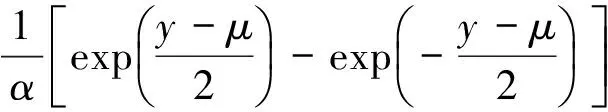
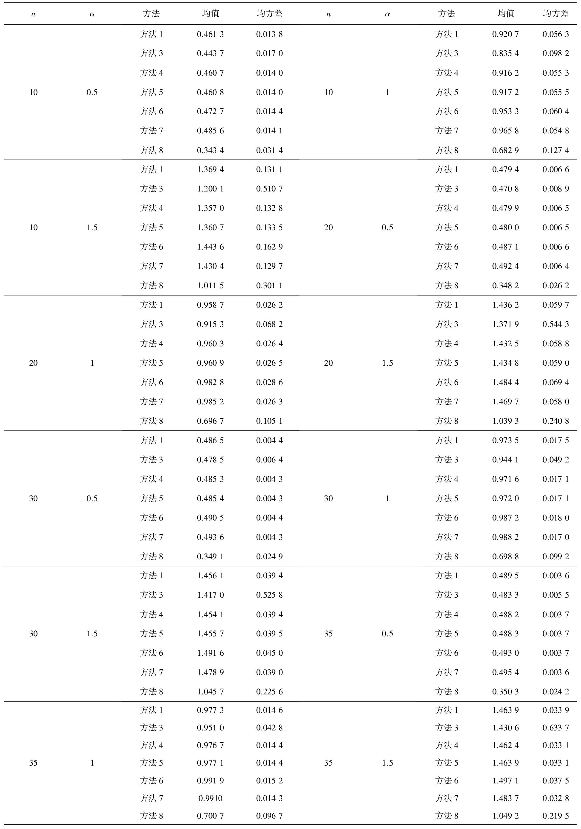
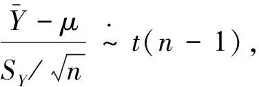
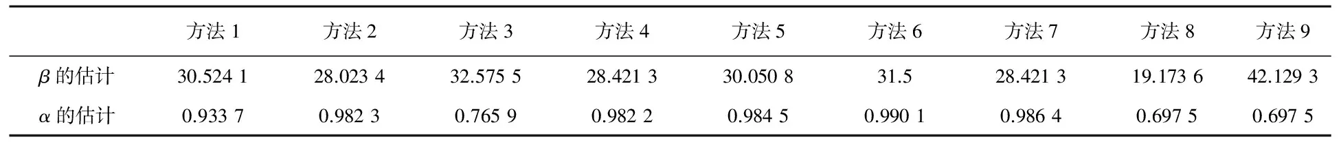
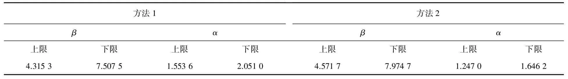
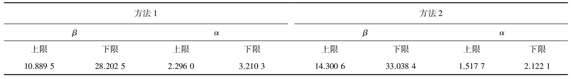
Y的分布函数FY(y)和密度函数fY(y)分别为： 对-∞

E(Y)=μ+2E(Z)=μ，

E(Y2)=μ2+4E(Z2)=

引理1[30]设X1,X2,…,Xn是来自总体X的容量为n的一个简单随机样本，记E(X)=μ，D(X)=σ2<+∞，该总体X的4阶中心矩v4=E(X-EX)4有限，若函数h(x)的四阶导数存在且有界，则有

证明Y=2Z+μ,E(Y)=μ,Y-E(Y)=2Z，

则Y的一至四阶中心矩为：

v1=E[Y-E(Y)]=0，

v2=E[Y-E(Y)]2=4E(Z2)=

v3=E[Y-E(Y)]3=8E(Z3)=0，

v4=E[Y-E(Y)]4=16E(Z4)=

令函数h(x)=ex，h(x)的任意阶导数任为ex，则

易证上述方程有唯一正实根.

1.2 方法2： 参数的极大似然估计[2， 14]

似然函数为：

L(α,β)=

化简得仅含参数β的超越方程：

需要指出的是，极大似然估计需要解非线性方程组，且计算较为复杂.

1.3 方法3： 矩估计

作简单运算，可得BS(α,β)分布的如下特征.

引理2[14]设随机变量T～BS(α,β)，则

(1)T-1～BS(α,β-1)；

化简得仅含参数α的超越方程：

6α4+8α2+4=cα4+4cα2+4c，

即 (c-6)α4+4(c-2)α2+4(c-1)=0，

Δ=16(c-2)2-16(c-6)(c-1)=

16(3c-2)>0，

又 (c-2)2-(3c-2)=c2-7c+6=

(c-1)(c-6).

要使方法3的矩估计存在，则样本数据应满足： 1

表1 10 000次模拟中满足c≥6的次数

Table 1 The number that satisfies c≥6 in 10 000 times of simulations

1.4 方法4： 矩估计

从中可解得参数β,α的矩估计分别为：

1.5 方法5： 逆矩估计

文献[15]给出了参数的逆矩估计如下：

1.6 方法6： 分位数估计

设T1,T2,…,Tn为来自Birnbaum-Saunders疲劳寿命分布总体T～BS(α,β)的一个容量为n的简单随机样本，其次序统计量记为T(1)≤T(2)≤…≤T(n).

进而参数α的点估计可取为

1.7 方法7： 回归估计

文献[21]利用回归分析模型，给出了如下参数的最小二乘估计：

1.8 方法8： 回归估计

由于

则

进而，

1.9 方法9： 回归估计

由于

1.10 参数点估计的模拟及比较分析

比较上述9种点估计方法，方法2由于涉及复杂的超越方程求解，在此不推荐使用.

下面通过10 000次Monte-Carlo模拟比较方法1、方法3～方法9的β点估计的精度.给定样本容量n=10,20,30,35，参数α=0.5,1,1.5，β=1，通过10 000次模拟得参数β的估计均值与均方差(其中方法3都满足1

(1) 固定n，随着α的增大，参数β估计的均值与真值的偏差增大，均方误差也增大；

(2) 固定参数α的真值，参数β的估计随着n的增加变精确；

(3) 方法1，4，5中参数β估计的无偏性较为明显，同时其均方误差也较小，相对而言，方法4的均方误差更小，方法5与方法1均方误差很接近.

下面通过10 000次Monte-Carlo模拟，比较方法1、方法3～方法8(方法9与方法8同)的α点估计的精度.给定样本容量n=10,20,30,35，参数α=0.5,1,1.5，β=1，通过10 000次模拟得参数α的估计均值与均方差(其中方法3都满足1

(1) 固定α，随着n的增大，参数α估计的均方误差在减少，即估计变精确；

(2) 方法1、方法4～方法7的均方误差相差不大，考虑到其均值，使用方法6或方法7更合理.

2 参数区间估计的比较分析

首先，给出利用对数正态分布求参数的区间估计方法(记为方法2)，进而通过Monte-Carlo模拟与文献[20-21]的方法(记为方法1)比较分析(在方法1能得到刻度参数β的区间估计的前提下).

记参数μ=lnβ，令Y=lnT,Yi=lnTi，i=1,2,…,n，则Y1,Y2,…,Yn为来自分布函数为

的一个容量为n的简单随机样本，其次序观察值记为y1,y2,…,yn.

表2 方法1、方法3～方法9参数β估计的Monte-Carlo模拟比较

Table 2 Comparisons on estimation methods 1, 3, 4,…, 9 of parameter β by Monte-Carlo simulations

表3 参数α估计方法的Monte-Carlo模拟比较

Table 3 Comparisons on estimation methods of parameter α by Monte-Carlo simulations

此时，

进而参数β的置信水平1-γ的近似区间估计为

参数α的置信水平1-γ的近似区间估计为

下面通过10 000次Monte-Carlo模拟，比较方法1、方法2关于参数α,β的区间估计的优劣.给定样本容量n=5,10,15，参数α=0.5,1,1.5，β=1，置信水平1-γ=0.90，通过10 000次模拟(方法1中的参数β的区间估计都存在)得参数α,β区间估计的平均下限、平均上限、平均长度，以及区间估计包含参数真值的次数，结果列于表4.可知方法1、方法2所得的区间估计包含参数的真值次数都大于9 000；方法2所得的区间估计的平均长度较方法1要短.可知方法2比方法1更优.

表4 参数区间估计的模拟比较

Table 4 Simulation comparisons of interval estimations of parameters

表5 例1的参数点估计

Table 5 Point estimations of parameters in example 1

3 计算实例

例1[14]数据来自BJERKEDAL(1960), 也被GUPTAETAL(1997)分析过.数据表示几内亚猪注射不同剂量结核杆菌的生存时间.几内亚猪对结核杆菌的敏感性比人类更高，首先关注在相同笼子里用相同养殖法养殖的猪.对于文中的养殖方法，有如下72个观测值：

12，15，22，24，24，32，32，33，34，38，38，43，44，48，52，53，54，54，55，56，57，58，58，59，60，60，60，60，61，62，63，65，65，67，68，70，70，72，73，75，76，76，81，83，84，85，87，91，95，96，98，99，109，110，121，127，129，131，143，146，146，175，175，211，233，258，258，263，297，341，341，376.

经计算得：c=1.651 2,d=0.063 1.

取置信水平为0.90，

利用区间估计方法1、方法2得参数β,α的置信水平为0.90的区间估计，如表6如示.

表6 例1的参数区间估计

Table 6 Interval estimations of parameters in example 1

例2[7]本实例中的数据集为6061-T6铝合金的疲劳寿命.铝合金的切取位置应平行于轧制方向，振荡频率为18 Hz.该数据集包括101个观测值，最大应力为31 000 Pa.数据如下：

70， 90， 96， 97， 99，100，103，104，104，105，107，108，108，108，109，109，112，112，113，114，114，114，116，119，120，120，120，121，121，123，124，124，124，124，124，128，128，129，129，130，130，130，131，131，131，131，131，132，132，132，133，134，134，134，134，134，136，136，137，138，138，138，139，139，141，141，142，142，142，142，142，142，144，144，145，146，148，148，149，151，151，152，155，156，157，157，157，157，158，159，162，163，163，164，166，166，168，170，174，196，212.

经计算得：c=1.027 7,d=0.003 6.

表7 例2的参数点估计

Table 7 Point estimations of parameters in example 2

表8 文献[7]中参数的其他几种点估计

Table 8 Other point estimations of parameters in reference[7]

文献[7]还给出了其他几种估计：

取置信水平为0.90，

取置信水平为0.95，

利用区间估计方法1、方法2得参数β,α的置信水平为0.90,0.95时的区间估计，如表9如示.

表9 例2的参数区间估计

Table 9 Interval estimations of parameters in example 2

例3[31]对于空气污染物浓度，假定数据不相关且相互独立，因此，一昼夜或循环趋势分析是无必要的.这一假设得到了很多学者(包括GOKHALE和KHARE等)的支持.例如，环境数据有时以均值作为指标，因此空间-时间依赖性不复存在.以下数据对应的是1973年5～9月纽约每日的臭氧浓度(由纽约州环境保护部提供)： 41，36， 12，18，28，23，19， 8， 7，16，11，14，18，14，34，6，30，1，11，4，32，23，45，115，37，29，71，39，23，21，37，20，12，13，49，32，64，40，77，97，97，85，10， 27，7，48，35，61，79，63，16，108，20，52，82，50，64，59，39，9，16，78，35，66，122，89，110，44，65，22，59，23，31，44，21，9，45，168，73，76，118，84，85， 96，78，91，47，32，20，23，21，24，44，21，28，9，13，46，18，13，24，16，23， 36，7，14，30，14，18，20，11，135，80，28，73，13.

表10 例3的参数点估计

Table 10 Point estimations of parameters in example 3

经计算得：c=1.607 8,d=0.092 8.

取置信水平为0.90，

利用区间估计方法1、方法2得参数β,α的置信水平为0.90时的区间估计，如表11如示.

表11 例3的参数区间估计

Table 11 Interval estimations of parameters in example 3

例4[32](1) 第1个实例是有关洪水峰值的超过数，含1958～1984年共72个超过数，四舍五入到小数点后1位，数据如下：

1.7，2.2，14.4，1.1，0.4，20.6，5.3，0.7，1.9，13.0，12.0，9.3，1.4，18.7，8.5，25.5，11.6，14.1，22.1，1.1，2.5，14.4，1.7，37.6，0.6，2.2，39.0，0.3，15.0，11.0，7.3，22.9，1.7，0.1，1.1，0.6，9.0，1.7，7.0，20.1，0.4，2.8，14.1，9.9，10.4，10.7，30.0，3.6，5.6，30.8，13.3，4.2，25.5，3.4，11.9，21.5，27.6，36.4，2.7，64.0，1.5，2.5，27.4，1.0，27.1，20.2，16.8，5.3，9.7，27.5，2.5，27.0.

经计算得：c=2.001 2,d=0.247 5.

表12 例4第1个实例的参数点估计

Table 12 Point estimations of parameters in the first case of example 4

取置信水平为0.90，

利用区间估计的方法1、方法2得参数β,α的置信水平为0.90时的区间估计，如表13如示.

表13 例4第1个实例的参数区间估计

Table 13 Interval estimations of parameters in the first case of example 4

(2) 第2个实例是有关50个工业设备的使用期，时间为零时进行寿命测试，数据如下：

0.1，0.2，1，1，1，1，1，2，3，6，7，11，12，18，18，18，18，18，21，32，36，40，45，46，47，50，55，60，63，63，67，67，67，67，72，75，79，82，82，83，84，84，84，85，85，85，85，85，86，86.

经计算得：c=1.506 2,d=0.382.

取置信水平为0.90，

利用区间估计方法1、方法2得参数β,α的置信水平为0.90时的区间估计，如表15如示.

表14 例4第2个实例的参数点估计

Table 14 Point estimations of parameters in the second case of example 4

表15 例4第2个实例的参数区间估计

Table 15 Interval estimations of parameters in the second case of example 4

[1] BIRNBAUM Z W, SAUNDERS S C. A new family of life distribution[J].JournalofAppliedProbability, 1969, 6(2)： 319-327.

[2] DESMOND A F. Stochastic models of failure in random environments[J].CanadianJournalofStatistics, 1985, 13(3)： 171-183.

[3] DESMOND A F. On the relationship between two fatigue-life models[J].IEEETransactionsonReliability, 1986, 35(2)： 167-169.

[4] BIRNBAUM Z W, SAUNDERS S C. Estimation for a family of life distributions with applications to fatigue[J].JournalofAppliedProbability, 1969, 6(2)： 328-347.

[5] ENGELHARDT M, BAIN L J, WRIGHT F T. Inferences on the parameters of the Birnbaum Saunders fatigue life distribution based on maximum likelihood estimation[J].Technometrics, 1981, 23(3)： 251-256.

[6] RIECK J R, NEDELMAN J R. A log-linear model for the Birnbaum Saunders distribution[J].Techanometrics, 1991, 33(1)： 51-60.

[7] NG H K T, KUNDU D, BALAKRISHNAN N. Modified moment estimation for the two-parameter Birnbaum-Saunders distribution[J].ComputationalStatisticsandDataAnalysis, 2003, 43(3)： 283-298.

[8] DUPUIS D J, MILLS J E. Robust estimation of the Birnbaum-Saunders distribution[J].IEEETransactionsonReliability, 1998, 47(1)： 88-95.

[9] CHANG D S, TANG L C. Reliability bounds and critical time for the Birnbaum-Saunders distribution[J].IEEETransactionsonReliability, 1993, 42(3)： 464-469.

[10] RIECK J R. Parametric estimation for the Birnbaum-Saunders distribution based on symmetrically censored samples[J].CommunicationinStatistics-TheoryandMethods, 1995, 24(7)： 1721-1736.

[11] OWEN W J, PADGETT W J. A Birnbaum-Saunders accelerated life model[J].IEEETransactionsonReliability, 2000, 49(2)： 224-229.

[12] OWEN W J, PADGETT W J. Acceleration models for system strength based on Birnbaum-Saunders distribution[J].LifetimeDataAnalysis, 1999, 5(2)： 133-147.

[13] OWEN W J, PADGETT W J. Power-law accelerated Birnbaum-Saunders life models[J].InternationalJournalofReliabilityQualityandSafetyEngineering, 2000, 7(7)： 1-15.

[14] KUNDU D, KANNAN N, BALAKRISHNAN N. On the hazard function of Birnbaum-Saunders distribution and associated inference[J].ComputationalStatistics&DataAnalysis, 2008, 52(5)： 2692-2702.

[15] 王炳兴，王玲玲. Birnbaum-Saunders疲劳寿命分布的参数估计[J].华东师范大学学报：自然科学版, 1996(4)： 10-15.

WANG B X, WANG L L. Parameter estimation of Birnbaum-Saunders fatigue life distribution[J].JournalofEastChinaNormalUniversity：NaturalSciences, 1996(4)： 10-15.

[16] 王炳兴，王玲玲. Birnbaum-Saunders疲劳寿命分布在截尾试验情形的统计分析[J].应用概率统计, 1996, 12(4)： 369-375.

WANG B X, WANG L L. Statistical analysis of Birnbaum-Saunders fatigue life distribution in the censored test case[J].AppliedProbabilityandStatistics, 1996, 12(4)： 369-375.

[17] 王蓉华，费鹤良. 双边截尾场合下BS疲劳寿命分布的参数估计[J].上海师范大学学报：自然科学版, 1999, 28(2)： 17-22.

WANG R H, FEI H L. Parameter estimation for the BS fatigue life distribution under bilateral censoring[J].JournalofShanghaiNormalUniversity：NaturalSciences, 1999, 28(2)： 17-22.

[18] WANG R H, FEI H L. Statistical analysis for the Birnbaum-Saunders fatigue life distribution under multiply type II censoring[J].ChineseQuarterlyJournalofMathematics, 2006, 21(1)： 15-27.

[19] WANG R H, FEI H L. Statistical analysis for the Birnbaum-Saunders fatigue life distribution under type II bilateral censoring and multiply type II censoring[J].ChineseQuarterlyJournalofMathematics, 2004, 19(2)： 126-132.

[20] 孙祝岭. Birnbaum-Saunders疲劳寿命分布尺度参数的区间估计[J].兵工学报, 2009, 30(11)： 1558-1561.

SUN Z L. Interval estimation of scale parameter for Birnbaum-Saunders fatigue life distribution[J].ActaArmamentarii, 2009, 30(11)： 1558-1561.

[21] 孙祝岭. Birnbaum-Saunders 疲劳寿命分布参数的回归估计方法[J].兵工学报, 2010, 31(9)： 1260-1262.

SUN Z L. Regression estimation method of parameters for Birnbaum-Saunders fatigue life distribution[J].ActaArmamentarii, 2010, 31(9)： 1260-1262.

[22] 孙祝岭. 疲劳寿命分布变异系数的统计推断[J].质量与可靠性, 2013(1)： 13-15.

SUN Z L. Statistical inference of variable coefficient for fatigue life distribution[J].QualityandReliability, 2013(1)： 13-15.

[23] 孙祝岭. Birnbaum-Saunders分布环境因子的置信限[J].强度与环境, 2012, 39(4)： 51-55.

SUN Z L. Confidence limit of environmental factor for Birnbaum-Saunders distribution[J].Structure&EnvironmentEngineering, 2012, 39(4)： 51-55.

[24] WANG B X. Generalized interval estimation for the Birnbaum-Saunders distribution[J].ComputationalStatisticsandDataAnalysis, 2012, 56(12)： 4320-4326.

[25] NIU C Z, GUO X, XU W L, et al. Comparison of several Birnbaum-Saunders distributions[J].JournalofStatisticalComputationandSimulation, 2014, 84(12)： 2721-2733.

[26] 周磊，孙玲玲. 一种基于概率解释的新型互连线时延Slew模型[J].电路与系统学报, 2009, 14(2)： 7-10.

ZHOU L, SUN L L. A new slew interconnect delay model based on probability interpretation[J].JournalofCircuitsandSystems, 2009, 14(2)： 7-10.

[27] 赵建印，孙权，彭宝华，等. 基于加速退化数据的BS分布的统计推断[J].电子产品可靠性与环境试验, 2006, 24(1)： 11-14.

ZHAO J Y, SUN Q, PENG B H,et al. Statistical inference for BS distribution based on the accelerated degradation data[J].ElectronicProductReliabilityandEnvironmentalTest, 2006, 24(1)： 11-14.

[28] BALAKRISHNAN N, ZHU X J. On the existence and uniqueness of the maximum likelihood estimates of the parameters of Birnbaum-Saunders distribution based on type-I, type-II and hybrid censored samples[J].Statistics, 2014, 48(5)： 1013-1032.

[29] 徐晓岭，王蓉华，顾蓓青. 关于两参数Birnbaum-Saunders疲劳寿命分布统计分析的2个注记[J].浙江大学学报：理学版, 2016, 43(5)： 539-544.

XU X L, WANG R H, GU B Q. Two notes of statistical analysis about two-parameter Birnbaum-Saunders fatigue life distribution[J].JournalofZhejiangUniversity：ScienceEdition, 2016, 43(5)： 539-544.

[30] 徐晓岭，王蓉华.概率论与数理统计[M]. 北京： 人民邮电出版社, 2014： 48-52, 174-178.

XU X L, WANG R H.ProbabilityandMathematicalStatistics[M]. Beijing： Posts and Telecom Press, 2014： 48-52, 174-178.

[31] VILCA F, SANTANA L, VICTOR LEIVA V, et al. Estimation of extreme percentiles in Birnbaum-Saunders distributions[J].ComputationalStatisticsandDataAnalysis, 2011, 55(4)： 1665-1678.

[32] CORDEIRO G M, LEMONTE A J. The exponentiated generalized Birnbaum-Saunders distribution[J].AppliedMathematicsandComputation, 2014, 247： 762-779.

XU Xiaoling1, WANG Ronghua2, GU Beiqing1

(1.SchoolofStatisticsandInformation,ShanghaiUniversityofInternationalBusinessandEconomics,Shanghai201620,China; 2.MathematicsandScienceCollege,ShanghaiNormalUniversity,Shanghai200234,China)

Statisticalanalysisoftwo-parameterBirnbaum-Saundersfatiguelifedistributionunderfullsample. Journal of Zhejiang University(Science Edition),2017，44(6)： 692-704

The logarithmic moment estimations of parameters are proposed by logarithmic transformation for two-parameter Birnbaum-Saunders(BS) fatigue life distribution BS(α,β) under the full sample. The precisions of various point estimation methods are compared by a large number of Monte-Carlo simulations. Two-parameter BS fatigue life distribution BS(α,β) is approximately regarded as two-parameter lognormal distribution through the first order Taylor expansion based on logarithmic transformation. Then, the approximate interval estimations of two parametersα,βare obtained, and it can be found that this approximate method is more accurate than the original method by Monte-Carlo simulations. Finally, several examples show the feasibility of the methods.

two-parameter Birnbaum-Saunders fatigue life distribution; shape parameter; scale parameter; point estimation; approximate interval estimation

2016-12-07.

国家自然科学基金资助项目 (11671264).

徐晓岭(1965—)，ORCID: http//orcid. org/0000-0002-9442-8555，男，博士，教授，主要从事应用统计研究，E-mail：xlxu@suibe.edu.cn.

*通信作者： ORCID: http//orcid. org/0000-0003-1539-8747，E-mail：gubeiqing@suibe.edu.cn.

10.3785/j.issn.1008-9497.2017.06.008

O 213

A

1008-9497(2017)06-692-13