
Tracer advection in an idealised river bend with groynes *
2018-10-27 09:10MohammadMahdiJalaliAlistairBorthwick
水动力学研究与进展 B辑 2018年5期
Mohammad Mahdi Jalali, Alistair G.L.Borthwick
Institute for Energy Systems, School of Engineering, The University of Edinburgh, Edinburgh, UK
Abstract: This paper presents numerical simulations of particle advection in the bend of an open channel containing groynes, which is an idealised form of a shallow river bend in a wide river.The flow field is computed using a boundary-fitted solver of the non-orthogonal, curvilinear shallow water equations.The computational grid is generated by solving Poisson-type elliptic partial differential equations using an iterative multi-grid scheme for prescribed boundary coordinates.The shallow water equations are discretised with finite differences in space, and 4th order Runge-Kutta integration in time.Tracers introduced at specific initial locations have their trajectories computed using Lagrangian particle tracking.The numerical shallow flow model is verified by comparison to the analytical solution of fully developed flow in an open channel.The combined shallow flow and Lagrangian particle-tracking model is then used to simulate the advection of tracer particles in a rectangular channel containing a pair of parallel groynes, and tracer particles in a curved open channel containing groynes, of dimensions roughly equivalent to a Danube River bend.
Key words: Shallow water equations, tracer advection, Lagrangian particle, curvilinear coordinates system, river bend, groynes
Introduction
Curved lateral boundaries and morphological features in a river affect the flow, and may reduce flood capacity at a river bend after increased runoff from extreme rainfall and snowmelt events.Enhanced sedimentation may occur at river bends due to increased depositional processes as a flood subsides.Moreover, river sediment deposited after flood inundation may have major societal, economic, and environmental repercussions, and so is an important factor in flood risk management.In practice, groynes are used to trap river sediment, prevent bank erosion,and attenuate the flow in large rivers[1].Although groynes have advantages regarding reduced flood risk,they are expensive to construct and maintain, and can affect navigation because of flow separation leading to the formation of turbulent eddies and larger-scale recirculation zones.It is therefore a challenge for engineers to design groynes that control the river,while meeting flood risk, navigation and economic cost objectives.A particular case of interest is the Danube River in Europe, where the advection and dispersion of sediment particles is known to be particularly complicated in the vicinity of groynes[2]and other hydraulic control structures[3].In large rivers,mixing occurs as a combination of local advection and dispersion processes that are enhanced in strongly sheared flows, such as turbulent eddies generated by flow separation at obstacles such as bridge piers and projecting groynes, and by roll-up of the bed boundary layer into hairpin vortices.Species transport is greatly affected by mixing, and influences water quality[4].Field observations, laboratory studies, and numerical simulation all offer insights into advection and mixing processes in large rivers[1].
Over the past forty or so years, considerable effort has gone into the development of river flow models that can accommodate complicated domains with curved and/or irregular boundaries.A variety of grid generation methods have been proposed[5]including structured rectangular and curvilinear,boundary-fitted grids, unstructured grids and sliding grids.Of the various methods available for grid generation, structured boundary-fitted grids are particularly appealing for shallow water applications in domains where the flow boundaries conform approximately to smooth curves.Boundary-fitted grids are generated by mapping an arbitrary-shaped domain onto a simple rectangular shape, or a series of interconnected rectangles[6].Johnson and co-workers[7-8]developed the first solvers of the shallow water equations on orthogonal grids.Borthwick and Barber[9]solved the non-orthogonal shallow water equations with Cartesian velocity components for jet-forced flow in a circular reservoir.Curvilinear grid approaches are used routinely nowadays for simulations of shallow flow hydrodynamics by means of single layer and multi-layer models, such as encapsulated in Delft3D for example.
Meanwhile particle-tracking methods, which involve the introduction of discrete particles into the flow domain and the numerical integration of the pure advection equation, have also been extensively utilised in water quality modelling of large rivers.In the context of chaotic advection near a groyne structure, Weitbrecht et al.[3]used 2-D particle tracking to examine advection in a rectangular channel flow with groynes.From a laboratory perspective,Zsugyel et al.[2]utilised PIV to examine the nonlinear trajectories of particles near a groyne in a rectangular channel.
The present study uses a curvilinear shallow flow numerical solver to simulate steady state flow fields in a curved open channel, and, with the aid of bilinear interpolation of the velocity field, uses Lagrangian particle tracking to simulate advection and mixing processes in the vicinity of a groyne inserted in the channel bend.The dimensions of the channel and groyne, and the flow conditions, are selected to be roughy similar to those in an idealised bend of the River Danube in Hungary.
1.Boundary-fitted grid generator
The boundary-fitted grid generator involved iterative solution of a pair of elliptic partial differential equations derived from the following Poisson equations that map between the Cartesian and curvilinear coordinate systems[6]:
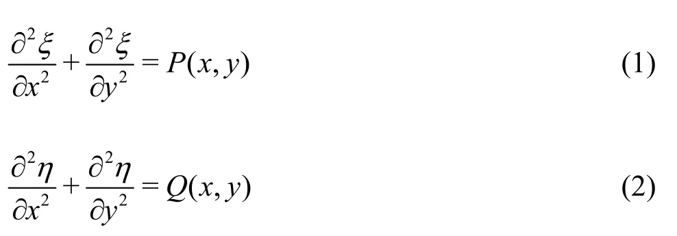
wherexandyare Cartesian co-ordinates in the physical plane,ξandηare curvilinear, boundaryfitted coordinates in the transformed plane, andPandQare expressions used to concentrateξ-lines andη-lines, if required.Using the chain rule, the governing Poisson equations are transformed from the Cartesian system to the curvilinear, boundary-fitted system where the boundaries form a rectangle in transformed system.Lettingthen the Jacobian ofxandywith respect toξandηis denoted byJ= ∂ (x,y) /∂(ξ,η).The resulting transformed grid generation equations are:
in which

The elliptic grid generation Eqs.(3)-(4) are solved as a boundary value problem, after discretization using second-order central differences and rearrangement to give:
xco-ordinate

yco-ordinate


where the subscriptsiandjdenote nodal positions in the transformed mesh, and the transformed mesh incremental lengths Δξand Δηare taken to be unity for convenience.In order to generate the grid,Equations (5), (6) are solved iteratively using the multi-grid technique[10], with boundary values prescribed as coordinates demarking the channel walls and open boundaries.
2.Shallow water equations
The shallow water equations are commonly used to model free surface, environmental flows where the depth is shallow, waves are long, and vertical motions of the water are sufficiently small that they may be neglected (i.e., hydrostatic pressure is assumed).The shallow water equations may be derived by depthintegration of the Reynolds-averaged continuity and Navier-Stokes momentum equations that are obtained from mass and momentum balances across an elemental volume.We denote the total depth ash=hs+ζ,wherehsis the still water depth andζis the free surface displacement in the vertical direction above still water level.Definingzas the vertical elevation above still water level, the continuity equation obtained as the incompressible version of the mass conservation equation is depth-integrated from the bed atz= -hsto the free surface atz=ζ, given

where,andare the Reynolds-averaged mean fluid velocity components in the Cartesianx,yandzdirections.Introducing depth-averaged velocity components in the Cartesianx,ydirections (satisfying the first mean value theorem of integration)

and applying Leibnitz’s formula for differentiation of an integral, and applying free surface and bed boundary conditions, the mass conservation shallow water equation is obtained as
in whichtis time.Similar depth-integrations are performed to derivexandyshallow water momentum equations, as follows.The depth-integrated form of the Reynolds-averaged Navier-Stokes momentum equations may be expressed

and

wherefis the Coriolis coefficient,σx′xandσy′yare deviatoric stress components, andτyx,τzx,τxyandτzyare shear stress components,ρis the density of water, andpis the pressure.Application of the Leibnitz rule and the kinematic bed and free surface boundary conditions gives (after some manipulation)

and


in whichτwx,τwyare the surface (wind) stress components, andτbx,τbyare bed stress components(which are usually evaluated using empirical friction formulae).The dispersive terms,ρ-1(∂/represent horizontal momentum exchanges due to the depth-averaging process.Their effect is usually expressed by means of momentum correction factors,β1,β2andβ3which can be calculated for a given boundary layer profile foruandv, and then subsumed into the corresponding advective acceleration term to give
and
where primes indicate fluctuating velocity components.To simplify the analysis, effective stresses may be defined as
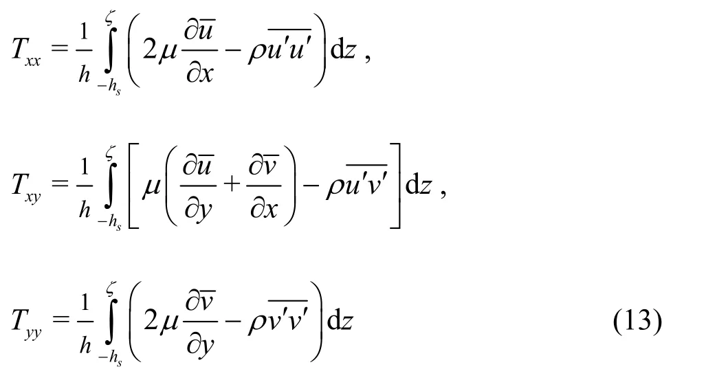
The effective stresses have two terms: the first relates to viscous stresses, the second to the turbulent Reynolds stresses.Replacing the Reynolds stresses by the Boussinesq approximation, the effective stresses become (noting thatε≫v, and making an approximation for the depth-averaged eddy viscosity)

Substituting for the effective stresses, invoking the dynamic pressure boundary condition that the pressure at the free surface is atmospheric, and assuming a hydrostatic pressure distribution with depth, we obtain the shallow water momentum equations, as:
wheregis the acceleration due to gravity,τwxandτwyare the wind stress components in thexandydirections, andτbxandτbyare the bed stress components in thexandy-directions.
The chain rule is used to transform the shallow water Eqs.(9), (15a) and (15b) from the Cartesian(x,y) system to the curvilinear (ξ,η) system,following Thomson et al.[6].The basic transformation relations may be written:
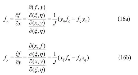
wherefis a differentiable function ofxandy,Jis the Jacobian, and subscript notation is used for differentiation.The transformed shallow water equations are then obtained[9]as:


and

where

The transformed shallow water equations are solved on a boundary-fitted grid, whose lines are defined such thatξ=iΔξandη=jΔη, wherei=1,2,…imaxandj= 1,2,…jmax, Δξand Δηare grid intervals in theξ- andη-directions, and timet=kΔt.The transformed shallow water Eqs.(17),(18a) and (18b) are discretized using second-order finite differences in space and a fourth-order Runge-Kutta scheme in time.The discretized version of the transformed equations may be summarized as follows:


With a suitable initial flow field and appropriate boundary conditions (slip conditions for walls, and prescribed (Dirichlet) or transmissive (van Neumann)conditions at open boundaries, the numerical model marches forward in time evaluating the finite difference form of the right hand side of Eqs.(20),(21a) and (21b).The fourth-order Runge-Kutta scheme is used to carry out the time integration implied by the right hand side of the equations.
3.Lagrangian particle tracking
The Lagrangian particle-tracking scheme simply involves numerical integration in time of the following advection equations

The Lyaponov exponent may be evaluated as a measure of mixing, after computing the mean particle separation distance of an initial array of particles as it evolves in time.In the present work, particles that have north and south adjacent particles are first selected.Then the mean particle separation is estimated, and plotted against time.
4.Results
4.1 Particle mixing in a rectangular channel containing a pair of parallel groynes
The coupled shallow water and particle-tracking model was used in the companion paper[11]to simulate particle advection in a rectangular open channel of length 3 600 m, width 300 m, and mean depth 1 m,which contains a pair of groynes.At the inlet open boundary, the velocity is set to 0.5 m/s.The eddy viscosity coefficient is 0.5 m2/s throughout the domain.The computational grid is 360 (stream-wise) by 30(transverse), the time step is 5 s, and the total flow simulation time is 4 000 s.Here, we extend the results to examine mixing processes by quantifying the degree of particle spreading with time.Figure 1 shows the mean particle separation distance as a function of time obtained for 54 000 particles that are initially uniformly spaced throughout the domain in red, blue,magenta, green, and yellow bands of equal width spanning the channel from south to north (for more information, see Fig.9(a) of the companion paper[11]).It is clear that the purple and green layers achieve the highest rates of dispersion.This is because they coincide with the wavy shear layer that is produced at the tips of the groynes, where the flow separates, and the mean flow drives recirculating zones in the lee of each groyne.

Fig.1 (Color online) Mean particle separation distance as a function of time for a rectangular channel containing two groynes and initially filled with particles that are uniformly distributed in coloured bands

Fig.2 Computational domains comprising 100×100 cell boundary fitted grids for 90° and 180° circular bends in open channels with inlet and outlet stems
4.2 Shallow flow model of idealised Danube River bends

Fig.3 (Color online) Shallow flow around 90° bend, with inlet and outlet stems: (a) Predicted and (b) Analytical steadystate velocity vectors, (c) Predicted and (d) Analytical velocity magnitude contours

Fig.4 (Color online) Shallow flow around 180° bend, with inlet and outlet stems: (a) Predicted and (b) Analytical steadystate velocity vectors, (c) Predicted and (d) Analytical velocity magnitude contours

Fig.5 (Color online) Predicted steady state velocity vectors in an open channel bend with two parallel groynes projecting from the inner boundary wall
The capability of the curvilinear shallow flow model to produce sensible flow hydrodynamics around an idealized bend was verified by considering idealized cases of shallow flow around 90° and 180°bends of inner radiusr0=1000mand outer radiusr1=1500m , with inlet and outlet stems both of which are 2 000 m long and 500 m wide.The water depth is 3 m, water density is 1 000 kg/m3, eddy viscosity is 9.3 m2/s and there is no wind stress present.Figure 2 shows the physical domains and the corresponding 100×100 grid used in both cases.The time step is 5 s,and the total simulation time is 5 000 s.Steady-state is achieved byt~ 2 500s .An analytical solution exists for streamlined flow around a circular bend.
Along the circular bend, the radial and tangential velocity components,uranduθ, are related to their Cartesian counterparts,uandv, by
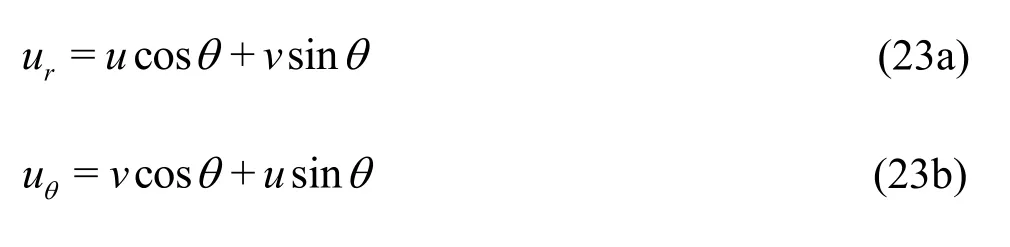
whereθis the polar angle.In the case of flow around a circular bend, a parabolic velocity distribution across the channel is obtained analytically,corresponding to fully developed flow in a channel[13]such that

whereuIis the mean flow speed at the inlet andr′is the distance measured radially from the midpoint of the channel.Figure 3 presents numerical predictions and analytical solutions of the steady-state velocity vectors and velocity magnitude contours for fully developed shallow flow around a 90° bend, with inlet and outlet stems.Figure 4 shows the corresponding results obtained for the 180° bend.In both cases, the model predictions and analytical solutions are in reasonable agreement.
4.3 Particle mixing in a groyned open channel bend
The coupled curvilinear shallow flow and particle-tracking model is next used to study tracer advection in an open channel comprising a 90° bend with inlet and outlet stems.The bend has interior radius of 3 300 m and an exterior radius of 3 600 m.Both stems are 3 600 m long and 300 m wide.The inlet flow velocity is set at 0.5 m/s, the downstream water depth to 1 m, and the eddy viscosity is 0.5 m2/s.

Fig.6 (Color online) Particle advections in an open channel bend with two parallel groynes, particles introduced immediately upstream of the first groyne

Fig.7 (Color online) Particle advections in an open channel bend with two parallel groynes, particles introduced between the first and second parallel groynes

Fig.8 (Color online) Predicted steady state velocity vectors in an open bend with two groynes projecting alternately from the inner and outer walls of the bend
The combined grid consists of a rectangular portion of 360×30 grid points covering the inlet stem,a 472×30 boundary-fitted grid for the circular bend,and a further 360×30 grid for the outlet stem.Stable results are achieved using a time step of 5 s, and steady state is reached well before the simulation ends at 5 000 s.Two cases are considered involving a pair of groynes projecting out from the channel wall into the mainstream: one where the groynes are located in series along the inner boundary, the other where the groynes are staggered with the upstream groyne projecting from the inner wall, and the other with the groyne projecting from the outer wall.
Figure 5 shows the steady state velocity vectors in a portion of the river bend for the first case where the two groynes are located in series.Recirculation zones occur in the lee of each groyne.From the Lagrangian particle-tracking model, it is possible to observe the effect of these recirculation zones on the trajectories taken by tracer particles.Figure 6 shows the dispersive transport of three bands of coloured tracers introduced immediately upstream of the first groyne, at 1 000 s intervals after the initial release until 5 000 s is reached.The green particles are advected rapidly by the through-flow beyond the ends of the groynes, whereas the blue particles are pulled towards the inner wall under the unfluence of the recirculation zone.The red particles creep across the first groyne and some become trapped within the recirculation zone.Figure 7 shows that similar results are obtained when the colour bands of tracer particles are introduced between the first and second parallel groynes.Here particles accumulate in the recirculation zone and particles are trapped by gyres downstream of the first groyne.Figures 8, 9 and 10 present the corresponding results obtained for the second case,when the groynes are arranged in a staggered configuration.Figure 8 shows the steady state velocity vectors.Flow separation occurs at end of each groyne,creating recirculation zones that serve to trap particles.Figures 9, 10 provide further visualizations of the tracer particle distributions when introduced as coloured arrays arranged in bands that are initially in front of the first groyne (Fig.9) and between the two groynes (Fig.10).Results are presented at intervals of 500 s after the initial release until 2 500 s.In the case of alternate groynes, the tracer particles are not trapped for as long as for the case of parallel groynes,and tend to be washed downstream except for those closest to a lateral wall.

Fig.9 (Color online) Particle advections in an open channel bend containing two alternate groynes, particles introduced immediately upstream of the first groyne
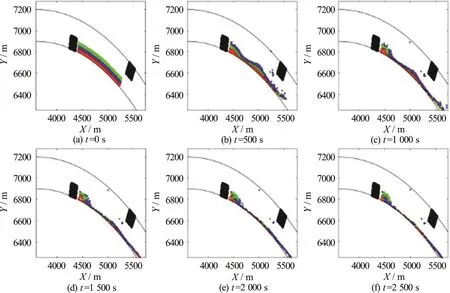
Fig.10 (Color online) Particle advections in an open channel bend containing two alternate groynes, particles introduced between the first and second parallel groynes
5.Conclusions
A primary reason for providing flood protection systems along rivers is to reduce flow speed and dissipate energy in the main channel through flow control devices.This paper has considered shallow flow in an idealised, curved open channel geometry representative of a Danube River bend.A coupled numerical model based on a boundary-fitted, curvilinear shallow flow solver and Lagrangian particletracking scheme predicted the shallow flow hydrodynamics in a curved open channel, and evaluated mixing of tracer particles.The model was applied to mixing in a rectangular channel containing two groynes in series oriented perpendicular to a lateral wall, showing that particles in the through-flow beyond the ends of the groynes mix less than those caught up in the shear layers and recirculation zones produced by the groynes.Close agreement was obtained between numerical and analytical predictions of the steady state velocity profiles produced by fully developed flow in a large bend, in the absence of groynes.
The coupled model was then applied to two cases of groynes in series and staggered configurations along an open channel bend.Use of bands of coloured particles highlighted the trapping effect of recirculation zones immediately behind the groynes.
Acknowledgement
The first author is grateful to the University of Edinburgh, which partly funded this research.

- 水动力学研究与进展 B辑的其它文章
- Call For Papers The 3rd International Symposium of Cavitation and Multiphase Flow
- Two-phase SPH simulation of vertical water entry of a two-dimensional structure *
- A selected review of vortex identification methods with applications *
- Simulation of the overtaking maneuver between two ships using the non-linear maneuvering model *
- The effect of downstream resistance on flow diverter treatment of a cerebral aneurysm at a bifurcation: A joint computational-experimental study *
- Nonlinear dynamic characteristics of a multi-module floating airport with rigid-flexible connections *