Experimental and numerical investigation of the influence of roughness and turbulence on LUT airfoil performance

Shoutu Li · Ye Li · Congxin Yang · Xiaobo Zheng · Qing Wang · Yin Wang · Deshun Li · Wenrui Hu

Abstract Vertical-axis wind turbines (VAWTs) have been widely used in urban environments, which contain dust and experience strong turbulence. However, airfoils for VAWTs in urban environments have received considerably less research attention than those for horizontal-axis wind turbines (HAWTs). In this study, the sensitivity of a new VAWT airfoil developed at the Lanzhou University of Technology (LUT) to roughness was investigated via a wind tunnel experiment. The results show that the LUT airfoil is less sensitive to roughness at a roughness height of ＜ 0.35 mm. Moreover, the drag bucket of the LUT airfoil decreases with increasing roughness height. Furthermore, the loads on the LUT airfoil during dynamic stall were studied at different turbulence intensities using a numerical method at a tip-speed ratio of 2. Before the stall, the turbulence intensity did not considerably affect the normal or tangential force coefficients of the LUT airfoil. However, after the stall, the normal force coefficient varied obviously at low turbulence intensity. Moreover, as the turbulence intensity increased, the normal and tangential force coefficients decreased rapidly, particularly in the downwind region of the VAWT.

Keywords Airfoil · Dynamic load · Roughness · Vertical-axis wind turbines (VAWTs) · Wind tunnel experiment

1 Introduction

Vertical-axis wind turbines (VAWTs) are widely used in urban environments. However, such environments contain dust and experience strong turbulence from natural wind [1, 2]. These factors can easily affect the dynamic load on the blades and the efficiency of VAWTs. In particular, strong turbulence is one of the main causes of dynamic stall [3]. Moreover, dynamic stall is complex, being considered as a delayed separation phenomenon on the airfoil surface due to unsteady motion of the wind turbine [4—6]. Therefore, dynamic loads on VAWTs during dynamic stall in urban environments must be clearly understood. The effect of dust on airfoil performance should also be investigated. Therefore, a considerable number of studies on VAWT development have focused on airfoil performance [7—10].

Compared with HAWTs, the local angle of attack (α) of VAWTs changes constantly with azimuthal angle (θ), even in a stable incoming airflow. Moreover, as the speed of rotation of the rotor decreases, the range of fluctuation of α increases. Previous research on VAWTs conducted by Ferreira et al. [9] and Islam et al. [11, 12] showed that the shape of the VAWT airfoil and the operating conditions played important roles in the dynamic stall phenomenon. They also offered some good suggestions for overcoming dynamic stall. Further analysis of the aerodynamic performance of VAWTs was conducted by Carrigan et al. and Howell et al. [13, 14] using a numerical method and wind tunnel experiments. Their results indicated that the performance of a VAWT could be improved by optimizing the airfoil profile. The effect of the airfoil on the performance of a VAWT was also described by Subramanian et al. [15] using a three-dimensional model. Therefore, studying the dynamic performance of new airfoils for VAWTs is important.

There is no doubt that roughness affects the aerodynamic performance of an airfoil [16—18], making such sensitivity to roughness one of the most important indices for assessing wind turbine airfoil performance. Early studies focused mainly on the mechanism underlying airfoil sensitivity to roughness. For instance, the process of boundary layer development on rough airfoils has been determined experimentally and through theoretical analysis [19, 20]. A great deal of meaningful work on airfoils for wind turbines was subsequently conducted [21]; For example, Timmer and Schaffarczyk [22] studied the performance of the DU-W-300Mod airfoil at high Reynolds number. Their research showed that the blunt trailing edge helped to decrease the roughness sensitivity of the airfoil. Similar work was also carried out by Zhang et al. [23], who investigated the aerodynamic performance of the S834 airfoil with different roughness heights using the shear stress transport (SST) k-ω turbulence model. Their results indicated that the sensitive height on the suction surface of the S834 airfoil was 0.5 mm, while the pressure surface was insensitive to the roughness height. Moreover, the sensitivity of thick airfoils to roughness has been extensively researched [22, 24], because roughness can easily increase the boundary layer thickness on a thick airfoil. This can cause the transition position to move toward the nose of the airfoil; For instance, Van Rooij and Timmer [25] reviewed the performance of many wind turbine airfoils, including the DU series, FFA series, AH series, S8xx, and NACA series, to assess the effect of roughness on thick airfoils. However, such studies have generally focused on the roughness sensitivity of airfoils at large Reynolds number (Re). Based on this literature review, more investigation on the influence of roughness on the performance of new airfoils is necessary.

The turbulence level also has a significant impact on the loads on and aerodynamic performance of VAWTs [2, 26, 27]. The fact that VAWTs experience a high degree of turbulence in urban environments cannot be ignored. To study the effect of turbulence intensity on VAWTs, Molina et al. [28] devised an innovative method to obtain highly turbulent wind conditions in a wind tunnel. They found that strong turbulence caused obvious vibrations and decreased the power of VAWTs. Similar work was performed by Ahmadi-Baloutaki et al. [29], who found that the power increased with a 5—10% increase in turbulence intensity. Moreover, VAWT self-starting was improved under the influence of free-stream turbulence. These results are similar to those obtained by Peng et al. [30] using large-eddy simulations and wind tunnel experiments. A numerical method was employed by Siddiqui et al. [31] to assess offshore wind energy, and their results indicated that the performance of VAWTs decreased by 23% to 42% for a 5% to 25% increase in turbulence intensity. The effect of turbulence on VAWT performance is therefore complex.

A new VAWT airfoil, known as the Lanzhou University of Technology (LUT) airfoil, was designed by our team. The LUT airfoil has a large maximum lift coefficient and thickness. High design lift and increased thickness generally heighten airfoil sensitivity to roughness [22, 32]. It was thus necessary and important to study the effect of roughness on the performance of the LUT airfoil. Relatively little research has been dedicated to VAWT airfoils in urban environments, and strong turbulence is an important cause of VAWT load instability. Therefore, we studied the dynamic loads on the LUT airfoil at different turbulence intensities. The remainder of this paper is organized as follows: Section 2 describes the experimental and numerical methods. Section 3 reports the sensitivity to roughness of and the dynamic loads on the LUT airfoil at different turbulence intensities.

2 Experimental and numerical methods

2.1 Experimental equipment and methods

The sensitivity of the LUT airfoil to roughness was investigated by measuring the airfoil surface pressure.

2.1.1 Wind tunnel

Airfoil surface pressure tests were carried out in a low-turbulence wind tunnel located at Northwestern Polytechnical University. As shown in Fig. 1, the rectangular cross-section of the experimental apparatus was 400 mm × 1000 mm, while its length was 2800 mm. The maximum wind speed was 70 m·s-1, and the turbulence intensity was below 0.3% . A more detailed description of the wind tunnel can be found elsewhere [33]. The x-, y-, and z-axes of the wind tunnel coordinate system represent the free stream, perpendicular direction, and span of the airfoil, respectively.

2.1.2 Test airfoil model

The LUT airfoil is an asymmetric VAWT airfoil with chord length (c) of 200 mm and span of 400 mm. A more detailed description of the LUT airfoil can be found in Ref. [34].

Fig. 1 Experimental wind tunnel: a schematic diagram; b photograph of experimental section. The cross-section of the wind tunnel was 400 mm × 1000 mm, with length of 2800 mm. The test model was the Lanzhou University of Technology (LUT) airfoil

Figure 2 shows how a total of 50 pressure taps with diameter of 0.7 mm were distributed on the surface of the model airfoil, concentrated at its leading and trailing edges. Carborundum no. 60 and no. 120 with average grain size of 0.30 mm and 0.12 mm, respectively, were used to ensure a fixed transition [20, 35]. The carborundum was attached to the upper and lower surfaces of the airfoil at positions corresponding to 10% and 15% of the chord length, respectively. It is worth noting that, because the carborundum was attached to the surface of the test airfoil using tape with height of 0.05 mm and width of 4 mm, the actual roughness heights were 0.35 mm (carborundum no. 60) and 0.17 mm (carborundum no. 120).

2.1.3 Pressure measurements

The pressure was measured using an electronic scanning measurement system (DSY104), a pressure scanner (PSI9816), and an angle-of-attack control mechanism. The pressure measurements and pressure scanning with the PSI9816 scanner were accurate to within ± 0.2% and ± 0.05% , respectively, of full scale (FS). The accuracy of angle-of-attack control was within ± 0.033°.

The pressure on the surface of the model airfoil is expressed as the pressure coefficientwhere piis the pressure at pressure tap i, p∞is the free-stream static pressure, U∞is the free-stream speed, and ρ is the air density. The drag coefficient was calculated using the wake investigation method. The height of the wake rake (H) was 300 mm. The wake rake was installed at a point 0.9c downstream from the trailing edge of the airfoil. The formula used to calculate the drag coefficient was

where y is the y-coordinate of the total pressure tap for the wake rake. The integral function of the wake rake is expressed as

Fig. 2 Distribution of pressure taps and locations of roughness tape on test model. Fifty pressure taps were distributed over the airfoil surface. Roughness tape is shown in green, attached on the upper surface at 0.1c and on the lower surface at 0.15c

The lift coefficient cLwas calculated based on the relationship between the coordinate system, the drag coefficient (cd), and the normal force coefficient cnas follows:

where α represents the angle of attack.

In the wind tunnel experiment, it was necessary to eliminate measurement errors. Therefore, the pressure values of the pressure taps and the wake rake were referenced to free-stream velocity of 0 m·s-1and angle of attack of 0°. The uncertainties on both the lift and drag coefficients were evaluated using the accuracy of the PSI9816 scanner.

2.2 Numerical method

Based on previous research [4, 5, 23], the unsteady Reynolds-averaged Navier—Stokes (URANS) method is considered reasonable and efficient for numerical analysis. In this work, the SST k-ω two-equation turbulence model of the URANS method was employed to simulate the dynamic performance of the LUT airfoil under free transition. The numerical simulations were carried out using ANSYS Fluent software (ANSYS, USA). The coupling of pressure and velocity was achieved using the SIMPLEC algorithm. The second-order upwind discretization scheme was utilized to calculate pressure and velocity, while the secondorder implicit formula was adopted to evaluate temporal discretization.

To calculate dynamic performance, the varying angle of attack was defined by the empirical Eq. (4) [37]:

where θ is the azimuthal angle and λ is the tip speed ratio.

The angular velocity (β) was defined by differentiating Eq. (4) with respect to time [4].

where t is the movement time, Ω is the angular frequency Ω=2πf , and f is the variation frequency of the angle of attack, which is typically f =0.55.

2.2.1 Boundary conditions and geometric schemes

Fig. 3 Schematic showing the geometry and boundary conditions of the numerical simulation. The diameter of the stationary zone was 40c, where c is the chord length, while the diameter of the rotating zone was equal to 6c. The regions on the left and right sides of the far domain are defined as a velocity inlet and pressure outlet, respectively

Figure 3 shows schematics of the boundary conditions and geometr y used for the numerical simulation. The aerodynamic center (0.25c) of the LUT airfoil, which was also the center of the rotational axis, was located at the origin of the coordinate system. The entire computational domain was divided into two parts. These included a stationary zone with diameter of 40c and a rotating zone with diameter of 6c, with an interface boundary condition set on the intersection of the two zones. The left region in the far domain was defined as a velocity inlet, where U∞= 23 m·s-1, while the region on the right was defined as a pressure outlet. The turbulence intensity and viscosity ratio were used to define the turbulence boundary conditions at the velocity inlet, with turbulence intensity of 0.14% , 10% , or 20% . The turbulence viscosity ratio was equal to 1, a typical value for the SST k-ω two-equation turbulence model. The backflow turbulence intensity and viscosity ratio of the pressure outlet boundary conditions were the same as those of the velocity inlet turbulence boundary conditions. The walls of the airfoil were set as no-slip walls.

2.2.2 Computational grid

Structured O-grids were adopted for the numerical simulation, as shown in Fig. 4. A sliding mesh was used for the rotating zone, which enables the required interpolation of flux to be obtained [4]. To ensure that y+was ＜ 1, the spacing of the first grid around the LUT airfoil was less than 1 × 10-5m.

Figure 5 shows the results of checking the mesh independence. The pressure coefficient on the LUT airfoil surface was investigated at an angle of attack (α) of 8° with a Reynolds number of 3 × 105. When the total number of cells exceeded 1.9 × 105, the results of the numerical simulation were in agreement with the reported experimental results. Therefore, the number of cells employed in the numerical method was greater than 2 × 105.

Fig. 4 Grid details around the rotating zone: a the O-grids employed and b the boundary layer comprising 36 cell layers. The height of the first layer was 1 × 10-6 m, and the growth rate of the grid in the boundary layer was 1.04

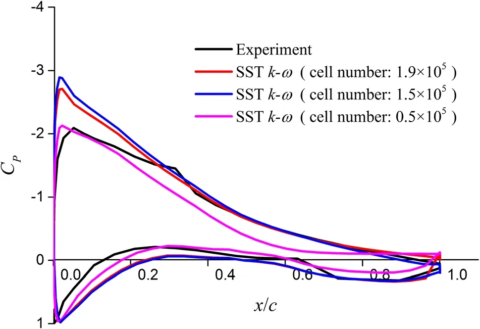
Fig. 5 Comparison of experimentally determined and numerical pressure coefficients on the LUT airfoil surface. Black, red, blue, and pink lines represent experimental results obtained with cell number of 1.9 × 105, 1.5 × 105, and 0.5 × 105, respectively. The angle of attack was 8°, and the Reynolds number was 3 × 105

Sufficient spatial resolution can ensure the accuracy of simulated airfoil dynamic performance. Therefore, it was necessary to study the effect of the time step in the numerical simulation. In this study, the time step was defined as [4, 38]

where τ is the dimensionless time step and Δt is the time step.

Table 1 presents the sensitivity to the dimensionless time step at a tip speed ratio of 2 when the numerical simulation was unsteady with a dynamic stall. Figure 6 shows the numerical LUT airfoil lift coefficients obtained with three different time steps under unsteady conditions with dynamic stall. The lift coefficient in case 3 was higher than those in cases 1 and 2 at the initial phase of stall during the upstroke process. Meanwhile, the numerical simulation for case 1 took less time than that of either case 2 or 3. Therefore, the time step in case 1 was adopted for numerical simulations to balance time and calculation accuracy.

Table 1 Sensitivity to the dimensionless time step

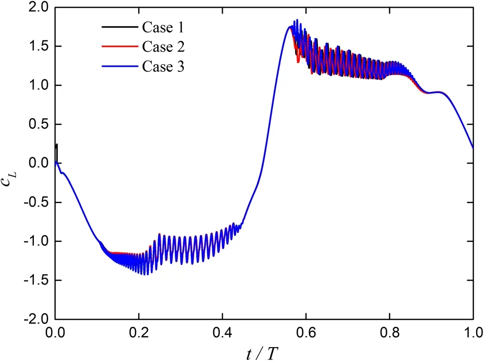
Fig. 6 Lift coefficients of LUT airfoil obtained by numerical simulation with different time steps at tip speed ratio of 2. Black, red, and blue lines denote the lift coefficient in case 1, case 2, and case 3, respectively

3 Discussion

The static pressure coefficient distribution on the LUT airfoil was obtained using different roughness heights in the wind-tunnel experiments. The dynamic loads on the airfoil were investigated at different turbulence intensities using the numerical method.

3.1 Effect of roughness on LUT airfoil performance

The sensitivity of the maximum lift coefficient, cL,max, to roughness was defined as [32, 39]

where cL,maxfris the maximum lift coefficient of a free transition and cL,maxfixis the maximum lift coefficient of a fixed transition.

3.1.1 Distribution of the pressure coefficients for various roughness heights

The experimentally determined pressure coefficients for the LUT airfoil at different angles of attack are shown for free and fixed transitions in Fig. 7. The black lines represent the pressure coefficients (cp) of the clean airfoil. The red and blue lines represent cpfor roughness height of 0.17 mm and 0.35 mm, respectively. Comparing the free and fixed transitions, at an angle of attack (α) of -10°, the effect of the roughness height on the pressure coefficient distribution was not obvious. When α = 4°, the location of the free transition on the LUT airfoil was at approximately 45% chord, while the pressure coefficient distribution on the upper surface clearly changed at about 20% chord due to the effect of the roughness height. With an increase in the angle of attack, the free-transition position moved towards the leading edge of the airfoil. Moreover, the pressure coefficient distributions on the upper and lower surfaces of the LUT airfoil were nearly identical at 12° angle of attack. At 16° angle of attack, the flow separation on the roughened upper surface was closer to the leading edge of the airfoil than it was on the clean airfoil. This can be seen in Fig. 7d. Additionally, the suction peak decreased with an increase in the roughness height, although the effect of the roughness on the lower surface was less obvious. Therefore, the effect of the roughness height on the LUT airfoil pressure distribution was weak before stall.

Fig. 7 Pressure distribution on LUT airfoil at different angles of attack in free and fixed transitions for a α = -10°, b α = 4°, c α = 12°, and d α = 16°. Black, red, and blue lines show the pressure coefficient for the clean case, roughness height of 0.17 mm, and roughness height of 0.35 mm, respectively

3.1.2 Lift coefficients at various roughness heights

The experimentally determined lift coefficients for the LUT airfoil with different roughness heights are shown in Fig. 8. The black lines indicate the lift coefficient of the clean airfoil, while the red and blue lines show the lift coefficients for roughness height of 0.17 mm and 0.35 mm, respectively. The variation in the lift coefficients was basically the same in all three cases before stall. Once the angle of attack exceeded 14°, the lift coefficients of the roughened airfoils dropped rapidly relative to the cLvalue of the clean airfoil. Stall began at 10° angle of attack, particularly for the airfoil roughened with 0.30 mm carborundum. In this case, the maximum lift coefficient was 15.65% lower than that of the clean airfoil. In other words, the sensitivity of the maximum lift coefficient (cL,max) to the roughness was 15.65% for the airfoil roughened with 0.30 mm carborundum. The sensitivity of the maximum lift coefficient of the airfoil roughened with 0.17 mm carborundum to roughness was 4% . Compared with the results of previous research [22, 32], cL,maxof the LUT airfoil was less sensitive to roughness.

3.1.3 Drag coefficients at various roughness values

The experimentally determined drag coefficients of the LUT airfoil for each roughness value are shown in Fig. 9. The black line represents the drag coefficient of the clean airfoil. The red and blue lines correspond to the drag coefficients at roughness height of 0.17 mm and 0.35 mm, respectively. Compared with the clean airfoil, the influence of roughness on the drag coefficient was quite minimal when - 7° ＜ α ＜ 9°. However, when the angle of attack exceeded 10°, the drag coefficients increased with increasing roughness. Consequently, the loss in momentum clearly became more pronounced as the roughness increased in the turbulent boundary layer. These results are consistent with the results discussed in Sect. 3.1.2.

3.1.4 Lift-drag ratio for various roughness values

The effect of the roughness height on the lift—drag ratio of the LUT airfoil is shown in Fig. 10, where the colors of the lines have the same meaning as in Fig. 9. In this figure, the variation of the lift coefficient with the drag coefficient for the LUT airfoil is complex, because the roughness height is so large that the momentum thickness increases [39]. Moreover, compared with the clean case, the width of the drag bucket decreases with increase in the roughness height.

3.2 Effect of turbulence intensity on LUT airfoil dynamics

Fig. 8 Lift coefficients of LUT airfoil with free and fixed transitions at Reynolds number of 3 × 105

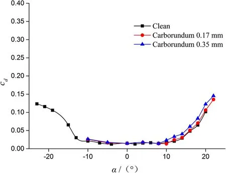
Fig. 9 Drag coefficients of LUT airfoil with free and fixed transition. Black, red, and blue lines show the drag coefficient corresponding to the clean case, roughness height of 0.17 mm, and roughness height of 0.35 mm, respectively, for Reynolds number of 3 × 105

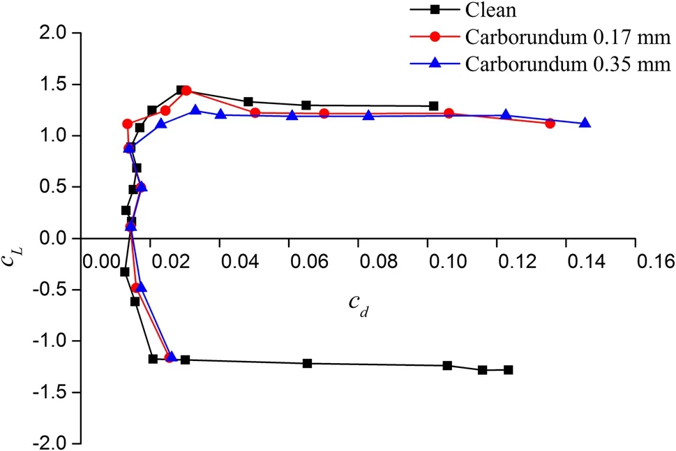
Fig. 10 Lift—drag ratios of LUT airfoil in free and fixed transitions. Black, red, and blue lines show the lift—drag ratios corresponding to the clean case, roughness height of 0.17 mm, and roughness height of 0.35 mm, respectively, for Reynolds number of 3 × 105

We investigated the dynamic properties of the LUT airfoil by performing numerical analysis of the normal and tangential force coefficients at turbulence intensity (TI) of 0.14% , 10% , and 20% , indicating low, moderate, and strong turbulence, respectively [4]. The nor mal force coefficient (cn) and tangential force coefficient (ct) were defined as follows:

where Fnis the normal force, Ftis the tangential force, and ρ is the air density.

The working principle of a VAWT is illustrated in Fig. 11a. The upwind area is defined by 0° ≤ α ≤ 180°, while the downwind area is defined by -180° ≤ α ≤ 0°. The variation in the angle of attack with the azimuthal angle according to Eqs. (4) and (5) is shown in Fig. 11b.

3.2.1 Effect of turbulence intensity on dynamic loads on LUT airfoil

The normal and tangential force coefficients of the LUT airfoil at different turbulence intensities and tip speed ratio of 2 are shown in Fig. 12a, b. During the upstroke process, when -16° ≤ α ≤ 22°, the normal force coefficient at the three turbulence intensities was nearly the same. However, the normal force coefficient clearly decreased when the angle of attack exceeded 22°, and it fluctuated when T I = 0.14% . When the angle of attack increased further, the fluctuation in the normal force coefficient was nearly the same in all cases. This indicates that the fluctuation in the normal force coeffi-cient could be delayed during stall as the turbulence intensity increases. In the downstroke process, when -12° ≤ α ≤ 30°, a similar variation in the normal force coefficient was observed at all three turbulence intensities. Therefore, strong turbulence after stall is advantageous for reducing fluctuations in the normal force coefficient. However, the normal force coefficient quickly dropped at the highest turbulence intensity. The turbulence intensity hardly affected the normal force coefficient prior to stall.

Fig. 11 Schematic illustration of vertical-axis wind turbine (VAWT): a two-dimensional cross-section and b variation in angle of attack with azimuthal angle at tip speed ratio of 2. The upwind area is defined by 0° ＜ α ＜ 180°, while the downwind area is defined by -180° ＜ α ＜ 0°. The circled numbers represent special positions in the period of motion. Lines shown with arrows denote the travel direction of the airfoil. F n is the normal force, F t is the tangential force, and θ is the azimuthal angle

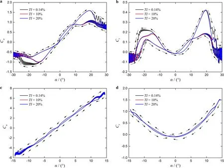
Fig. 12 Dynamic loads on LUT airfoil at different turbulence intensities at Reynolds number of 3 × 105: a normal and b tangential force coeffi-cients when λ = 2, c normal and d tangential force coefficients when λ = 4

In Fig. 12b, the tangential force coefficients at each turbulence intensity were similar in the region where -12° ≤ α ≤ 22° during the upstroke process. After stall, there was a downward trend in the tangential force coefficient, and it fluctuated in each case. However, fluctuation was observed earlier at TI = 0.14% . In the downwind region, where the angle of attack was negative, the tangential force coefficient exhibited the strongest fluctuations. The largest peak value was found in the case of TI = 0.14% , indicating that an increase of turbulence intensity caused a decrease in the maximum lift coefficient in this region. However, compared with the downstroke process, the effect of the turbulence intensity on the tangential force coefficient was weak in the upstroke stage.

Figure 12c, d displays the normal and tangential force coefficients of the LUT airfoil at the different turbulence intensities when the tip speed ratio was 4. They show that the changes in the normal and tangential force coefficients were almost the same at the different turbulence intensities. However, compared with Fig. 12a, b, the values of the normal and tangential force coefficients obviously increased when the tip speed ratio changed from λ = 2 to λ = 4 for the LUT airfoil. Meanwhile, the maximum value of the dynamic angle of attack decreased with increase of the tip speed ratio due to the weaker effect of the dynamic stall; this result can be explained based on Eq. (4).

Thus, the turbulence intensity did not affect the normal or tangential force coefficient at low tip speed ratio prior to stall. The effect of the turbulence intensity on the normal and tangential force coefficients was weak in the area upwind of the VAWT when stall occurred. Fluctuations in both the normal and tangential force coefficient decreased in the area downwind of the VAWT as the turbulence intensity increased. At the same time, the normal and tangential force coefficients themselves dropped quickly.

3.2.2 Effect of turbulence intensity on flow-field characteristics of LUT airfoil

The purpose of considering λ = 2 as an example is to further illustrate the dynamic characteristics of the LUT airfoil and investigate the development of the flow field of the LUT airfoil.

Figure 13 shows the instantaneous contours of the streamline and velocity of the LUT airfoil at different turbulence intensities when λ = 2 and the instantaneous velocity (U*) was equal to U*=U∕U∞. When TI= 0.14% , the flow on the upper surface of the LUT airfoil during the upstroke process (α = 12.1° ↑) remained attached. When the angle of attack increased, a tailing-edge vortex gradually formed and grew until α = 20.9° ↑. A larger tailing-edge vortex was also observed. Therefore, the normal and tangential force coeffi-cients changed almost linearly during this process, as shown in Fig. 12. As the angle of attack increased further, the larger tailing-edge vortex gradually moved to the leading edge along the upper surface of the LUT airfoil and shed from the upper surface. This process is clearly shown from α = 20.9° ↑ to α = 29.2° ↑. In this range of α, the normal and tangential force coefficients clearly fluctuated. In the downstroke process, the tailing-edge vortex on the lower surface was present until α = -11.8° ↓. Moreover, the vortex development was the same as that on the upper surface in the upstroke stage. However, the larger tailing-edge vortex fell off the lower surface at α = - 22.4° ↓.

The flow conditions around the LUT airfoil at a small angle of attack, e.g., α = 12.1° ↑, were the same regardless of the turbulence intensity. When the turbulence intensity increased, the intensity of the vortex near the trailing edge increased. An example is shown for α = 26.5° ↑. The distribution of the instantaneous pressure coefficients at different turbulence intensities during this process is shown in Fig. 14. The black lines correspond to the instantaneous pressure coefficients at TI = 0.14% . The red and blue lines represent the pressure coefficients at TI = 0.10% and TI = 20% , respectively.

At α = 12.1° ↑, the pressure coefficients were the same in all three cases. At α = 20.9° ↑, flow separation occurred on the upper surface of the LUT airfoil after x/c reached 0.27. At α = 26.5° ↑, the flow separation extended to x/c = 0.08. However, when TI = 0.14% and α = 20.9° ↑ or 26.5° ↑, the pressure coefficient showed a slight improvement over the other two cases. This result coincides with the trend shown in Fig. 12. At TI = 0.14% , the normal and tangential force coefficients were larger than they were at TI = 10% or 20% . The pressure coefficient near the trailing edge of the LUT airfoil was unstable when TI = 10% and TI = 20% .

However, the flow separation during the downstroke process, particularly at α = 30° ↓, was opposite to that of the upstroke process. Therefore, the tangential force coefficient at a negative angle of attack was higher at TI = 0.14% than at either TI = 10% or TI = 20% .

4 Conclusions

To evaluate the static and dynamic properties of the newly designed LUT airfoil, we tested the sensitivity of the airfoil to roughness and studied the effect of the turbulence intensity on its performance. We found t hat VAWTs with the LUT airfoil would be suitable for use in urban environments.

The roughness height affected the pressure coefficient, lift coefficient, and drag coefficient of the LUT airfoil at angles of attack greater than 14°. The sensitivity of the maximum lift coefficient of the airfoil at roughness height of 0.17 mm and 0.35 mm was 4% and 15.65% , respectively. Thus, the LUT airfoil was less sensitive to roughness. As the roughness height increased, the width of the drag bucket, stall angle, and maximum lift coefficient decreased. Moreover, the lift coefficient clearly decreased with an increase in the roughness height after stall.

Prior to stall, the effect of the turbulence intensity on the normal and tangential force coefficients of the LUT airfoil was weak in regions upwind (α ＞ 0°) and downwind (α ＜ 0°) of the VAWT. However, in the upwind region of the LUT airfoil in stall, the normal force coefficient appeared to fluctuate at low turbulence intensities. When the turbulence intensity increased, the normal force coefficient dropped rapidly and the fluctuation reduced. The variation in the normal force coefficient was similar in downwind and upwind regions. Compared with the normal force coefficient in upwind regions, the tangential force coefficient did not differ significantly with the turbulence intensity. However, the tangential force coefficient fluctuated more significantly at low turbulence intensities in downwind regions. Moreover, the fluctuation decreased as the turbulence intensity increased. Therefore, the turbulence intensity could affect the dynamic loads on the LUT airfoil after stall, particularly in downwind regions. The effect of the turbulence intensity on the normal and tangential force coefficients in upwind regions was comparatively weak.

In future work, the dynamic performance and noise level of the LUT airfoil will be tested in a wind tunnel experiment.

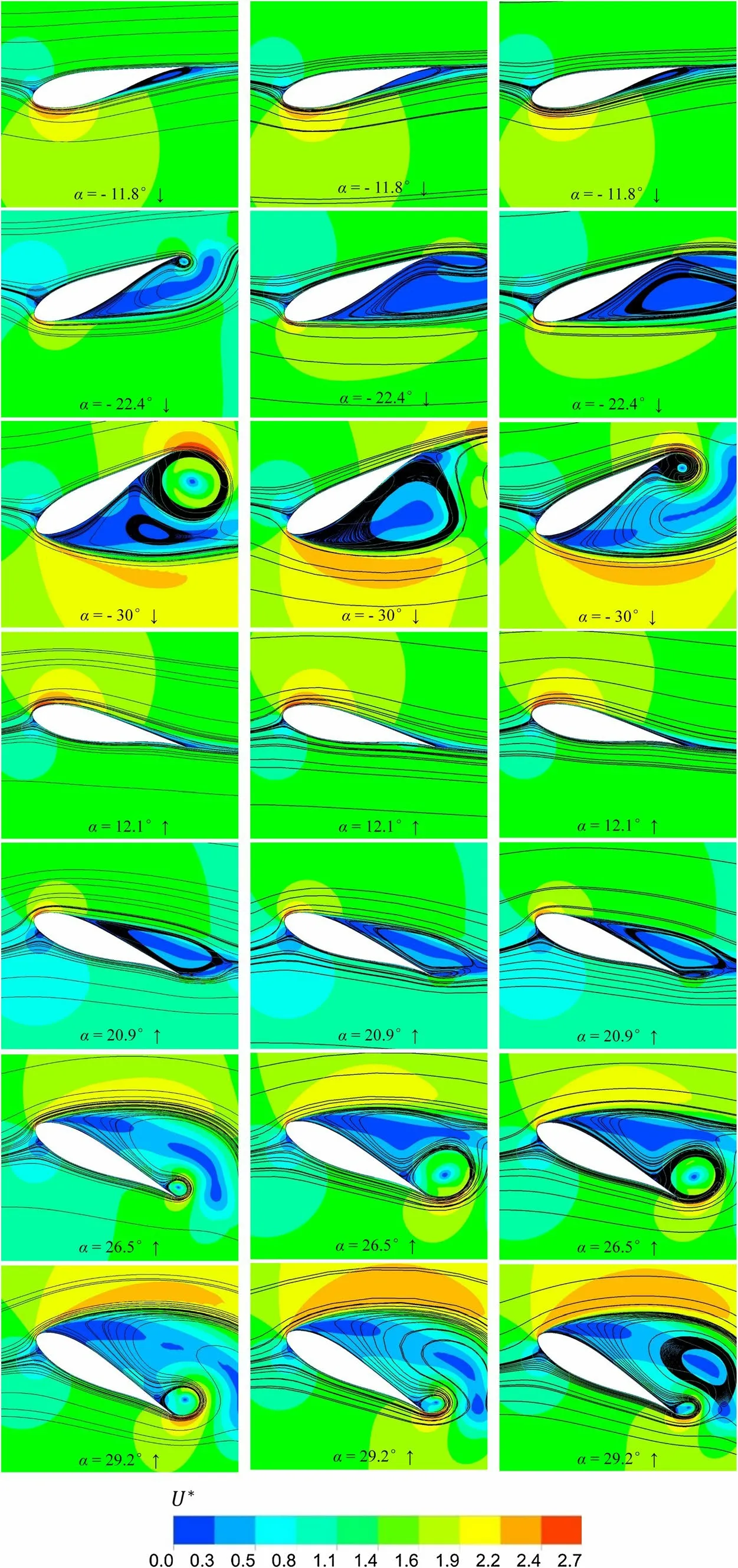
Fig. 13 Contours of instantaneous streamline and velocity of LUT airfoil at different turbulence intensities when λ = 2: a TI = 0.14% , b TI = 10% , and c TI = 20%

Fig. 14 Distribution of instantaneous pressure coefficients of LUT airfoil at different turbulence intensities when λ = 2: a α = 12.1° ↑, b α = 20.9° ↑, and c α = 26.5° ↑

AcknowledgementsThis work was supported by the Natural Science Foundation of GANSU (grant 1508RJYA098), National Natural Science Foundation of China (grants 51766009, 51761135012, 11872248), and National Basic Research Program of China (grant 2014CB046201). The authors also thank the people who provided many good suggestions for this paper, and Northwestern Polytechnical University for providing the experimental instruments and wind tunnel.