Connected Vehicle-Based Traffic Signal Coordination

Wn Li, Xuegng Bn

a Oak Ridge National Laboratory, Knoxville, TN 37932, USA

b University of Washington, Seattle, WA 98195, USA

Keywords:

Connected vehicles

Traffic signal coordination

Dynamic programming

Two-level optimization

Mixed-integer nonlinear program

ABSTRACT This study presents a connected vehicles(CVs)-based traffic signal optimization framework for a coordinated arterial corridor. The signal optimization and coordination problem are first formulated in a centralized scheme as a mixed-integer nonlinear program (MINLP). The optimal phase durations and offsets are solved together by minimizing fuel consumption and travel time considering an individual vehicle’s trajectories. Due to the complexity of the model, we decompose the problem into two levels:an intersection level to optimize phase durations using dynamic programming(DP),and a corridor level to optimize the offsets of all intersections.In order to solve the two-level model,a prediction-based solution technique is developed. The proposed models are tested using traffic simulation under various scenarios. Compared with the traditional actuated signal timing and coordination plan, the signal timing plans generated by solving the MINLP and the two-level model can reasonably improve the signal control performance. When considering varies vehicle types under high demand levels, the proposed two-level model reduced the total system cost by 3.8% comparing to baseline actuated plan. MINLP reduced the system cost by 5.9%.It also suggested that coordination scheme was beneficial to corridors with relatively high demand levels. For intersections with major and minor street, coordination conducted for major street had little impacts on the vehicles at the minor street.

1. Introduction

Over the past several decades, extensive efforts have been devoted to improving the performance of traffic signal control systems in order to alleviate ever-growing traffic congestion.Connected vehicle (CV) technologies have received increasing attention in signal timing optimization.These technologies include vehicle-to-vehicle (V2V) communication,vehicle-to-infrastructure(V2I)communication,vehicle-to-pedestrian(V2P)communication,and vehicle-to-everything (V2X) communication. CVs make it possible to collect drivers’ information, including their origins,destinations, and precise trajectory information (e.g., second-bysecond vehicle speeds and locations). Such information can be transferred to signal controllers for signal timing optimization.CVs can also benefit signal coordination for multiple intersections on a signalized corridor or a road network,which can provide efficient movements of vehicle platoons through adjacent intersections. There are three key parameters for signal coordination:cycle length, split, and offset. Cycle length is defined as the time period to finish a complete signal phase sequence. Coordinated traffic signals normally need to have the same cycle length, called the ‘‘common cycle length” (although half of or double the common cycle length is sometimes acceptable as well). In practice,such a common cycle length can be determined by signal design tools,such as SYNCHRO†† http://www.trafficware.com/synchro.html‡ https://trlsoftware.com/products/junction-signal-design/transyt/and TRANSYT‡† http://www.trafficware.com/synchro.html‡ https://trlsoftware.com/products/junction-signal-design/transyt/.Split is the sum of the green time and clearance time of a particular phase,which is a segment of the cycle length allocated to the phase. It is also called the phase duration. Offset is the time difference between a fixed point in the cycle of an intersection (e.g., the start of the green time) and a system reference point. Coordination is especially beneficial for intersections on a corridor, which are closely spaced to each other (e.g.,a spacing of 1200 m has been suggested by the US Federal Highway Administration (FHWA) [1]) and the traffic demands between adjacent intersections are relatively large and random.

Signal coordination models have some common measures of effectiveness (MOEs). Bandwidth maximization used to be a common objective function for signal coordination. It is the amount of time that a vehicle can travel through all intersections of the coordinated corridor without stopping.Bandwidth is related to the system capacity and to the throughput,which is determined by the offsets. The early literature on bandwidth optimization mostly relies on the graphical method [1-4], and the later literature focuses on mixed-integer linear programs (MILPs) to maximize the sum of the bandwidths for the two directions of the coordinated corridor [5]. Branch and bound algorithms are often used to solve the optimization problem. For example, Gartner et al.[6]expanded the previous signal coordination models by considering actual traffic volumes and flow capacity in the MILP formulation for bandwidth optimization. Their model is called MULTIBAND because they defined a different bandwidth for each direction of the corridor, which was individually weighted based on their contributions to the objective value. PASSER is a software tool developed to maximize the bandwidth efficiency, given precalculated splits [7]. Other measures of effectiveness include delays, total travel times, number of stops, and queues. Coogan et al. [8] optimized the offset of coordinated traffic signals to reduce the average queue lengths at all intersections by assuming a fixed timing plan with a common cycle length for each intersection.They derived a closed-form analytical model of a non-convex,quadratically constrained quadratic program (QCQP). The simulation results demonstrated a significant reduction in queue lengths.Due to the stochastic nature of traffic flows, travel time reliability is another important indicator to measure dynamic traffic conditions. Zheng et al. [9] considered minimizing average travel time and its reliability as the objective to optimize the fixed cycle length, effective green times, and offsets. They applied a geneticalgorithm-based approach to solve the nonlinear optimization problem.The proposed model was shown to significantly improve travel time reliability and reduce delay in a simulation network and a real-world corridor. Hu and Liu [10] developed a datadriven model to minimize the total delay for an arterial corridor.They solved two problems in the proposed model:the early return to green problems for the coordinated phase and the uncertainty of the intersection queue size. A commonly used method for network-level traffic signal optimization problems is the decomposition solution technique [11-15]. Although most decomposition methods do not consider offset as a variable in their model, they take advantage of the coordination properties when optimizing signal timing for a traffic network.The traffic signal timing of each intersection is determined by accounting for the influence of traffic conditions and signal timing in a large area,such as a few upstream and downstream intersections.As a result,multiple adjacent intersections are synchronized to improve system operations.

With the advent of CV technology,vehicles(drivers)and traffic infrastructure can exchange information in real time. Such information (e.g., origins, destinations, departure times, and secondby-second trajectories) can be used by the infrastructure to better update traffic signal timing in order to reduce congestion and improve fuel efficiency.Li et al.[16]developed a signal timing optimization and coordination model based on individual vehicle trajectories in the CV environment. Green times and offsets for multiple signals in a corridor were optimized in a mixed-integer nonlinear program (MINLP). Li and Ban [17] formulated the traffic signal optimization problem for a single intersection as an MINLP.It was then reformulated as a dynamic programming(DP)problem with a two-step method to ensure that the optimal green splits from the DP sum up to a fixed cycle length. Beak et al. [18] developed a two-level optimization model for adaptive coordination in the CV environment. At the intersection level, the optimal green time for each phase was determined from DP.At the corridor level,the offset was optimized to obtain the minimum delay. The proposed model can reduce the average delay and number of stops for both the coordinated phase and the entire network. Lee et al.[19] developed a real-time traffic signal control method in the CV environment based on cumulative travel time. Kalman filtering techniques were utilized to estimate the cumulative travel times under various CV penetration rates. These scholars suggested that the proposed method can be applied for signal coordination on a major street.Li et al.[20]developed a bi-level optimization model to optimize traffic signal timings in a network. The upper level of the model calculated the optimal green time and offsets to minimize the average travel time, while the lower-level problem was developed to achieve network equilibrium. These researchers decomposed the bi-level problem to a single-level problem solved by the genetic algorithm (GA) and dynamic traffic assignment(DTA).Priemer and Friedrich[21]proposed an adaptive traffic signal control method for multiple intersections in the CV environment. They applied DP and enumeration to optimize signal timing parameters in order to reduce the queue length for the next 20 s under various penetration rates of CVs. Islam and Hajbabaie[22] developed a distributed traffic coordination scheme. They reduced the complexity of a network-level decision problem to a single intersection level problem by deciding the termination or continuation of green times. They also evaluated the influence of the demand levels and penetration rates of CVs in several case studies.

At present, most traffic signal timing optimization and coordination methods apply a centralized scheme in which various signal timing parameters(phase durations,cycle lengths,and offsets)are optimized together in one mathematical problem.This can lead to several problems. First, individual vehicle-based traffic signal control/coordination problems often have large dimensions and are usually nondeterministic polynominal (NP)-complete (a class of computational problems for which no efficient solution algorithm can be found) [22]. Second, for a large traffic corridor or road network, signal timing optimization and coordination problems are difficult to solve and are not applicable for real-time signal control.Some scholars have tried to decentralize signal optimization problems by decomposing the entire problem into a few manageable sub-problems. However, these studies mostly used varying cycle lengths[19-22]and thus cannot be applied directly to traffic signal coordination.

This study aims to generate the optimal signal timing parameters of multiple adjacent intersections by taking advantage of V2I and V2V communications in the CV environment. All the vehicles in the corridor are assumed to be connected to the infrastructure(when they are within a certain distance of the intersection)so that their trajectories(second-by-second speed and location)are available in real time to signal controllers for signal timing optimization. In particular, we extend the signal optimization method of Li and Ban [17] from a single intersection to the optimization and coordination of multiple intersections on a traffic corridor. In order to account for the coordination of vehicles, the fixed cycle length constraint is applied to the problem. The overall CV-based signal control and coordination problem is first formulated as an MINLP. The objective is to minimize the fuel consumption and travel times of all CVs in the corridor by calculating the optimal phase durations and offsets at the same time. Since the MINLP model has a large dimension, directly solving the problem is challenging. Thus, we decompose the problem into a CV-based two-level traffic signal optimization and coordination scheme that contains an intersection level and a corridor level.In order to solve this two-level model,we develop a prediction-based approach that collects the arrival vehicle information at the beginning of each cycle and calculates the optimal phase durations for each intersection using a DP method proposed by the authors previously in Ref.[23]. During the calculation process, each intersection acknowledges the other intersections’ signal status, vehicle states, and‘‘temporary” optimal offsets. This ensures that the traffic flows on the main street are coordinated among adjacent intersections. At the corridor level,the‘‘temporary”offsets are calculated iteratively in order to find the optimal offsets when the total cost converges to its minimum.

The proposed model is different from the two-level optimization method developed by Beak et al. [18] in several important aspects. First, at the intersection level, Beak et al. applied a fixed force-off option and added more coordination constraints to the DP method to calculate signal timing parameters. Such a method is itself in a two-level structure, making the overall framework used by Beak et al. [18] essentially a three-level model. The proposed two-level model uses DP with the two-step method reported by Li and Ban [17,23] to calculate the optimal signal timings for a single intersection, which sums up to a fixed cycle length. At the corridor level, Beak et al. [18] developed an MILP to minimize the delay of a vehicle platoon. This paper accounts for the individual vehicle’s trajectories when determining the optimal offsets, and thus considers more detailed information than the corridor-level model in Ref. [18].

This study contributes to the literature in this field by:

(1)Formulating the traffic signal optimization and coordination problem as an MINLP accounting for individual CV trajectories on a signalized corridor;

(2) Reformulating the problem from a large-sized centralized optimization problem to a decentralized two-level signal control problem, with an intersection level to optimize the signal timing parameters of individual intersections and a corridor level to calculate the offsets;

(3) Proposing a prediction-based iterative solution method for the two-level problem.

2. Traffic signal coordination

Along a corridor or for a network, traffic coordination provides smooth progression for a platoon of vehicles traveling through multiple adjacent intersections. In this study, the objective is to calculate optimal traffic signal parameters—that is, phase durations and offsets—for a corridor by minimizing the fuel consumption and travel time of all CVs along the coordinated directions (i.e., on the main street). As shown in Fig. 1(a), we can treat the bottom intersection as the reference signal and coordinate the other intersections based on the signal operations of the reference signal.Usually,the offset value is maintained for a period(e.g.,30 min)and may be changed based on real traffic conditions.

We apply a dual ring controller in this study.The dual ring controller is comprised of six groups with a sequence of eight phases,as proposed in Ref. [23] and shown in Fig. 2(a). It is assumed that the through movements of eastbound (EB) and westbound (WB)are the coordinated directions (movements 2 and 6 in Phase 1 in Fig.2(b))and cannot be skipped for coordination purposes.Phases 2 and 3 cannot be realized at the same time because there are conflicting movements. The same rule applies for Phases 6 and 7 in phase group 5.

2.1. Formulating signal coordination as an MINLP

Fig. 1. Coordination of multiple intersections. (a) Schematic of a road with traffic coordination (numbers 1-8 represent different movements; E: east direction);(b) offset illustration (the distance between two intersections can be varies(e.g., 1000 m)).

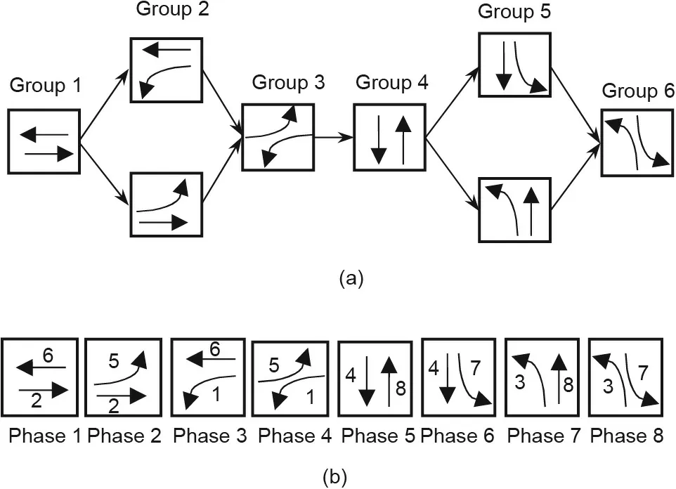
Fig. 2. Traffic signal configuration. (a) Traffic signal configuration in phase groups;(b) traffic signal configuration in phases.

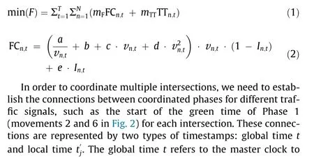
In the previous studies developed by the authors [17,23] the signal control problem for a single intersection is formulated as an MINLP. It can produce the optimal phase durations that satisfy the fixed cycle length constraint. This model is then extended to a corridor-level model by introducing a new variable, offset Ojfor intersection(signal)j,when considering the coordination of multiple intersections on the corridor. The objective is to minimize fuel consumption and travel time for all vehicles(where the total number of vehicles is N) on the corridor for the total time span T, as shown in Eq.(1).FCn，tand TTn，tare the fuel consumption and travel time for vehicle n at time t. The parameters mFand mTTare the monetary values. For example, mFcan be set as $0.8 USD per liter($3 USD per gal) and mTTis $12 USD per hour. Here, we apply the fuel consumption models developed by Zhao et al. [24], as shown in Eq. (2). Fuel consumption FCn，tis calculated based on vehicle speed vn，t.If a vehicle is idling(speed less than 8 km•h-1),the indicator variable for idle status,In，tis equal to 1;otherwise,it is 0.The fuel consumption parameters a, b, c, d, and e are calibrated based on various vehicle types, as shown by Zhao et al. [24].

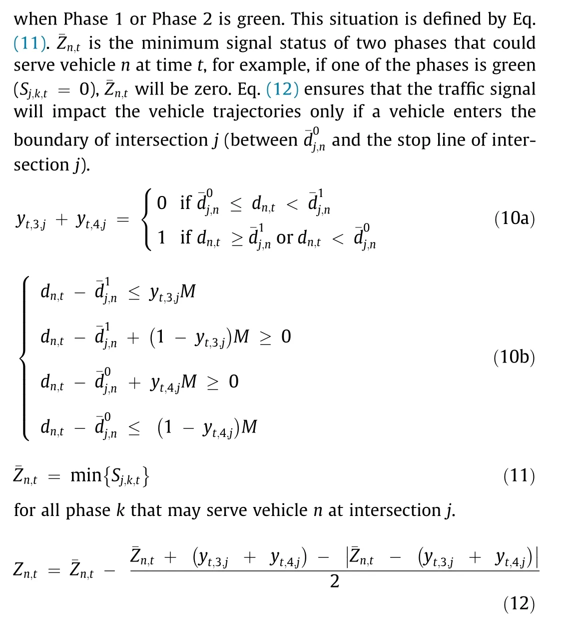
After the signal status for vehicle n has been identified, its trajectories can be estimated and predicted based on the intelligent driving model (IDM) [26]. In order to account for the influence of signal status on CVs,we model the traffic signal as a‘‘virtual vehicle.” When the signal status is red, it is a standing vehicle with a speed of 0 and a predefined location. When the signal is green, it disappears from the network. Eq. (13a) identifies whether the leader of vehicle n is a real vehicle or a‘‘virtual vehicle”by comparing the location of the nearest front traffic signal of vehicle n(dsignal，n) to the locations of vehicle n (dn,t) and vehicle n - 1(dn-1，t). Parameter dsignal，ndenotes the location of the nearest front signal of vehicle n. Eq. (13b) is equivalent to Eq. (13a) using big M method.

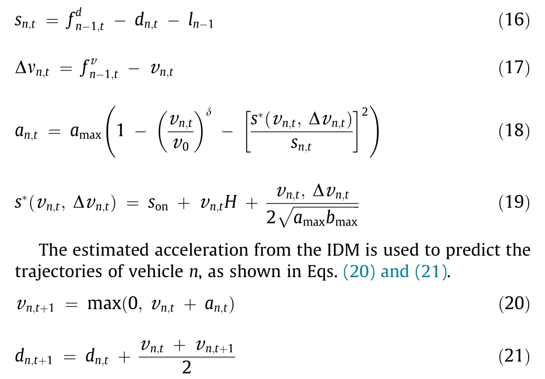
Eqs. (16)-(19) apply the IDM to calculate the acceleration an，tfor vehicle n at time t. Variable sn，testimates the vehicle gaps,ln-1denotes the vehicle length, Δνn，tdenotes the speed difference between vehicle n and its preceding vehicle v0is the vehicle desired speed, sonis the standstill vehicle gap, H denotes the desired time headway, and amaxand bmaxdenote the maximum acceleration and deceleration rate, respectively. The exponent δ is usually set as 4. See the work of Li and Ban [17,23] for more details.

Eqs. (1)-(21) provide the signal optimization and coordination model for multiple intersections in the CV environment. When the trajectories of each vehicle are considered, the model clearly shows that the problem can be formulated as an MINLP. The proposed model given in Eqs. (1)-(21) is a significant extension to the model in Ref. [23], while being much more complex. First of all,the number of variables is greatly increased,from eight phases for a single intersection to eight phases multiplied by the number of intersections, in addition to the newly added offset variables.Moreover,a road corridor or network contains many more vehicles than a single intersection;thus,the prediction of the vehicle trajectories—that is,their second-by-second speed and location over certain time periods and a certain network range—imposes an increased computational burden. Furthermore, the complex interactions between the status of each vehicle and the multiple traffic signals lead to various if-then-else conditions in the model (Eqs.(1)-(21)). The resulting MINLP formulation is even more difficult to solve and is not applicable for real-time signal control. In the next section, we present how to decompose the CV-based traffic signal optimization and coordination problem (Eqs. (1)-(21)) into a decentralized two-level model that can be solved more efficiently.

2.2. Reformulating signal coordination as a two-level model

Due to the complexity of the MINLP formulation(Eqs.(1)-(21)),we reformulate the MINLP as a decentralized two-level problem.In this two-level model, instead of solving the phase durations and offsets optimization for multiple intersections as one mathematical programming, we decompose the overall problem into two levels: an intersection level to optimize the phase durations for every single intersection, and a corridor level to optimize the offsets of all intersections. As a result, the complexity of the original mathematical model is largely reduced.

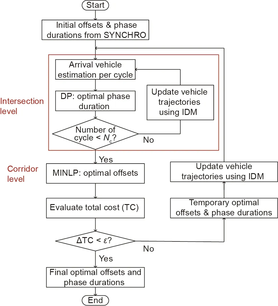
Fig. 3. Solution technique of the two-level traffic signal optimization model. Nc:certain number of cycles; ε: the threshold to determine if the corridor-level computation converges or not.

Fig.3 shows the overall framework of the two-level model.We assume that all intersections and vehicles are connected and that they can send messages to each other. We further assume that some initial offsets and phase durations are available; in this case,they are calculated in SYNCHRO 6†† http://www.trafficware.com/synchro.html., which is a well-known traffic signal optimization software. The vehicles arriving at each intersection can then be estimated and predicted using the IDM. In particular,the DP model with a two-step method[23]is applied to compute the optimal phase durations in every cycle of each intersection.This method is able to calculate the phase durations that satisfy the fixed cycle length constraint for a single intersection. Fig. 4 illustrates the acyclic graph of the DP method, which is equivalent to in order to find the shortest path in the graph. The variable offset provides the connection between the intersection- and corridor-level optimizations.In order to consider the influence of the offsets on the DP formulation for an intersection, we implement and solve the DP for intersection j using its local time,following Eq.(3).This essentially reduces the model(Eqs.(1)-(21))for the entire corridor to each individual intersection.For details of the DP method for a single intersection, refer to Ref. [23].

After the optimal signal plans for all intersections on the corridor are generated for a few cycles,the information is transferred to a central controller, where offset optimization is conducted at the corridor level.Usually,the offset values are maintained for a period of time and are not updated in every cycle. Here, we assume that the offsets will be updated for every certain number of cycles, Ncin Fig. 3; that is, Nccould be ten cycles. When the number of running cycles is greater than Nc, the intersection level computation terminates and process to corridor level. The parameter ε is the threshold to determine if the corridor-level computation converges or not,for example,ε could be 0.01.We further reformulate the offset optimization problems as an MINLP in this section, but with much fewer variables since the phase durations for each intersection are obtained by solving the intersection-level model above(using the DP method in Ref. [23]). The objective of the corridorlevel optimization is to minimize the fuel consumption and travel time of all CVs on the main street of the corridor:

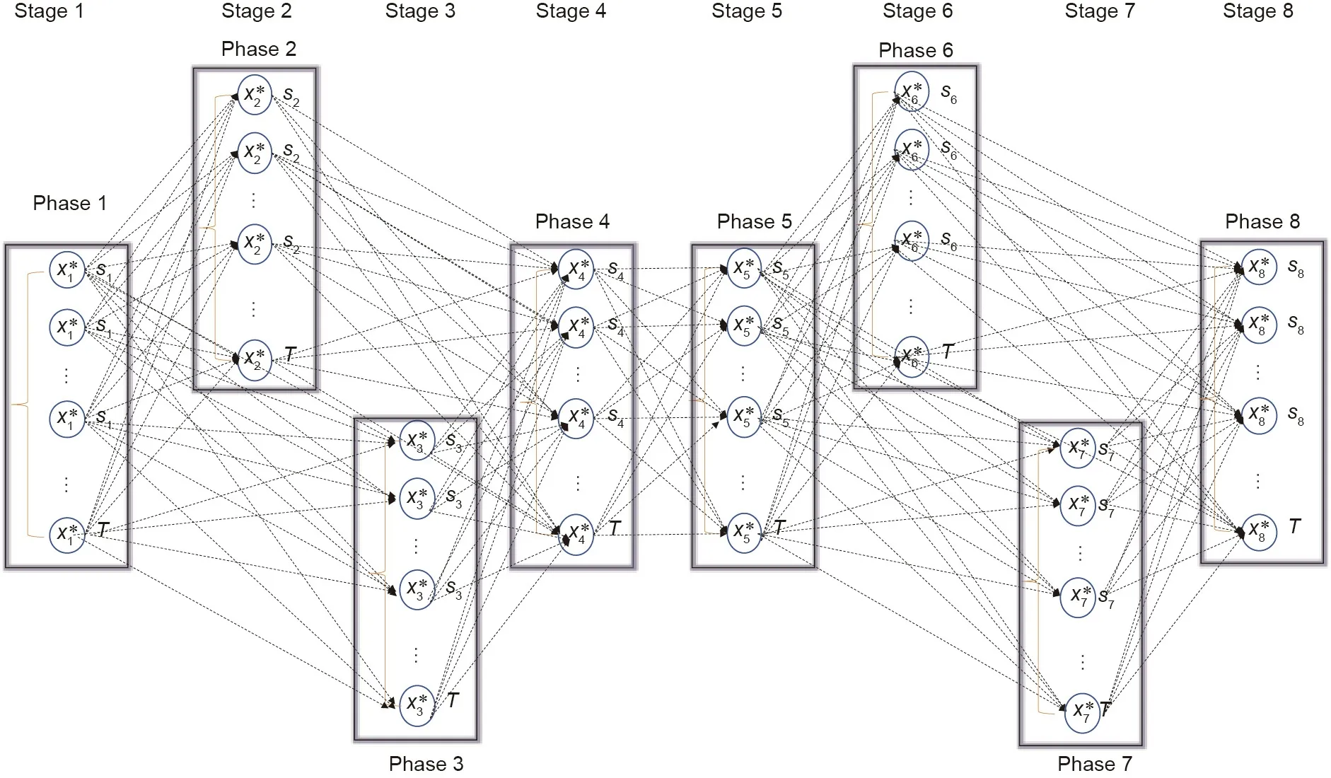
Fig.4. Acyclic graph of the DP method. denotes the optimal green time allocated to stage p;sp is the state variable representing the total time from the beginning of the horizon to the end of stage. The dotted arrows represent the stage processing sequence in DP.

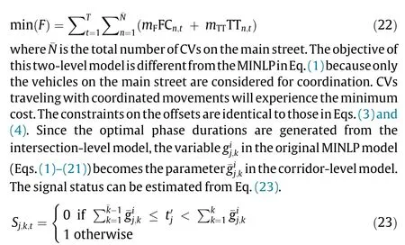
After the signal status is identified, the vehicle trajectories can be estimated from the IDM using Eqs. (10)-(21). In summary,Eqs. (10)-(23) constitute the corridor-level offset optimization model. It is also an MINLP, but with a much simpler dimension than the original MINLP (Eqs. (1)-(21)). The phase duration variables in the original MINLP are no longer variables in the corridor-level offset optimization model because they are already optimized in the intersection-level model using DP. The corridorlevel model can be solved by the NOMAD solver in Matlab [27].It computes/updates the vehicle speed and location at each time step using the IDM.As shown in Fig.3,in order to find the optimal offsets, ‘‘temporary” optimal offsets generated from the corridorlevel MINLP are calculated iteratively until the total cost converges.The convergence criterion is defined as the difference between the total costs estimated from two consecutive iterations—that is,when ΔTC is less than a small tolerance, such as 10-5.

3. Numerical experiments

The proposed traffic signal optimization, coordination models,and solution methods are tested in a simulation network that contains five signalized intersections in a corridor. The distance between two adjacent intersections is 800 m (0.5 mile). The WB and EB are the coordinated directions. The boundary of an intersection is defined as 400 m upstream and 400 m downstream of the stop line, as shown in Fig. 5. Vehicle arrivals are randomly generated at the boundary of the entire network, with known arrival times, initial speeds, and turning movements. We also assume that there is only one lane per incoming approach (plus the left-turn bay at the intersection), so no lane-changing behavior is modeled. The penetration rate for CVs is assumed to be 100%. There are three steps in evaluating the proposed methods and comparing their performance with those of other models.First,the optimal signal timing parameters,including cycle length,phase duration, and offset are calculated in SYNCHRO, under different traffic demand levels. Second, we apply different methods to calculate the optimal signal plans (phase duration and offset)for each case. Third, we compare the performances of all methods by implementing the calculated plans in the same simulation network.It is noted that SYNCHRO implements the fixed optimal signal plan (based on average traffic demand) for a certain time period, which does not account for an individual vehicle’s trajectories or for different vehicle types.In contrast,the proposed twolevel model accounts for real-time-arrival vehicle patterns, varied vehicle types, and the number of turning/through vehicles in the signal timing determination process by taking advantage of CV technologies.

We first test six cases that account for different traffic demand levels and vehicle types(Table 1),similar to those tested by Li and Ban[17,23].In Cases I-III,all vehicles are sedans.Vehicle demands for the main street westbound and eastbound (WE) directions are set from low (250 vehicles per hour (vph)) to high (800 vph). For the minor street northbound and southbound (NS) directions, the demands are set at 125,250,and 250 vph.In Cases IV-VI,the vehicle demand levels are identical to those in Cases I-III, while the vehicle types are set differently. All the vehicles in the NS directions are electric vehicles (EVs) and all the vehicles in the main directions WE are buses.In these six cases,80%of the CVs will use through movements and the other 20% will turn left at each intersection.

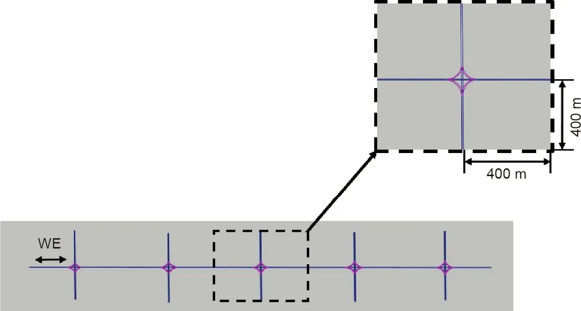
Fig. 5. Simulation network containing five intersections. WE: westbound and eastbound (the coordinated directions).

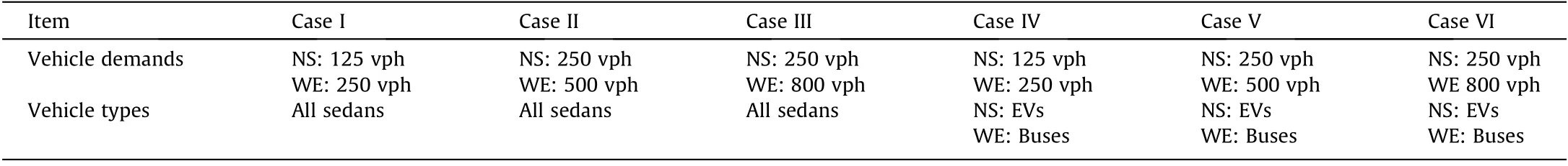
Table 1 Six cases of different traffic demand levels and vehicle types.

Table 2 shows the total costs estimated using different signal plans generated from the three methods in ten cycles(the minimal total cost for each case is highlighted). The first method is generated from SYNCHRO using an actuated traffic signal system.Given the geometric information of the corridors and volumes on each movement,SYNCHRO can calculate the optimal signal parameters,including phase durations, cycle lengths, and offsets. The optimal signal plan, together with information on the randomly generated arrival vehicles and updated trajectories using the IDM,are implemented in the simulation network to calculate the total cost—that is,Eqs.(1)and(2).Methods MINLP and two-level model in Table 2 follow the same procedures to calculate the cost.Note that we consider a fixed cycle length constraint in this study in order to conduct signal coordination. The cycle lengths for different cases are estimated using SYNCHRO—that is, 60 s for low traffic demand(Cases I and IV), 80 s for medium traffic demand (Cases II and V),and 120 s for high demand (Cases III and VI). The second method,the MINLP in Eqs.(1)-(21),is solved by the NOMAD solver in Matlab.There are eight phases for each signal,as shown in Fig.2.If signal plans are calculated in every ten cycles, there will be 40 variables of the phase durations and four variables of the offsets for the simulation network containing five signals. The third method is the proposed decentralized two-level model, which can be solved by the proposed prediction-based approach. At the intersection level, the phase durations for each intersection are solved by the DP method and can be updated every cycle. At the corridor level, the offsets are solved every ten cycles.

For all cases, the results from the MINLP and the two-level model are better than those from SYNCHRO. For Cases III and IV,the results from the two-level model are better than those from the MINLP. Fig. 6 shows the improvement in model performance for each case.In Cases I and IV,which have relatively low demand levels, the improvements are smaller than in the other cases; this finding may suggest that coordination will bring limited benefits when traffic is relatively light.

Apart from the total cost of travel time and fuel consumption,we also compare the number of stops among all methods in Tables 3 and 4. The number of stops for the coordinated movements are generally smaller than those for the other movements for all six cases. In addition, the number of stops generated from SYNCHRO are larger than those generated from the MINLP or the proposed two-level model.

To further evaluate whether coordination can benefit the entire network,including both the main street and the minor street under different scenarios,we compare the improvement in model performance between two scenarios: with coordination and without coordination(i.e.,offset value equals 0).For example,in the MINLP,we first solve the model that contains only 40 variables of the phase durations and set all offset values to 0. We then implement the estimated signal plan in the IDM and estimate the total cost for the main street and the minor street separately. These costs are compared with the results from solving the entire model (Eqs.(1)-(21)), which optimizes both the phase durations and the offsets. The same procedures are applied to the two-level model.Table 5 shows the comparison results. The negative values are highlighted in the table; they suggest that by applying coordination, the performance for the main street or the minor street becomes worse. For the main street, the MINLP and the two-level model both underperform under low demand levels (Cases I or IV)if applying coordination,while the improvements are more significant for higher demand levels (Cases II, III, V, and VI). The results suggest that coordination schemes may not be beneficial to a corridor with low traffic volumes and random arrival vehicles,because those vehicles are less likely to form a platoon to be influenced significantly by the operation of adjacent intersections. For the minor street,the improvements are relatively small,regardless of whether they are positive or negative.Coordination on the main street seems to have little impact on the vehicles on the minor street in these six cases.

Table 2 Total cost of three methods for six cases (Unit: USD).

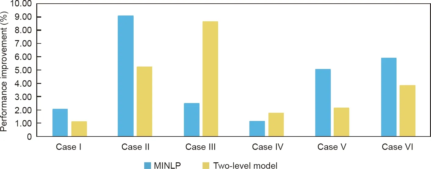
Fig. 6. Improvement in model performance over SYNCHRO for Cases I-VI.

Table 3 Number of stops for the coordinated movements.

Table 4 Number of stops for all movements.

Table 5 Model performance improvement with coordination for the main street and the minor street.

The previous six cases tested the influences of various combinations of demand levels and vehicle types on signal coordination.It is still worth testing how the proposed methods perform under various traffic demands in opposite directions or different movements (turning and through movement). Hence, three more cases(Cases VII-IX) are tested. First of all, the traffic demands for right-turn movements are added to the simulation network. The vehicles traveling on left-turn and right-turn movements are randomly sampled at between 10% and 20% of the total demands for each approach in Cases VII-IX. In addition, traffic demands in the opposite directions are not the same; for example, in the main street, the volumes in the E-W and W-E directions are different.For Cases VII and VIII, the traffic demand in each direction is a given value, as shown in Table 6. In Case IX, the traffic demand in each direction is randomly sampled within a certain range. For example, in the E-W direction, the initial demand is randomly(uniformly) selected from a range between 250 and 500 vph. In all cases, the performance of the MINLP and the two-level model are better than those of the baseline SYNCHRO model. The model improvements are shown in Fig. 7.

Fig.8 shows the vehicle trajectories updated based on different signal plans for ten cycles (600 s) along a 4000 m corridor. The vehicles are traveling in the W-E direction in Fig.5.Compared with the trajectories generated using the SYNCHRO plan in Fig.8(a),the delays and number of stops in Figs. 8(b) and (c) are significantly reduced by applying the MINLP method and the two-level model.Through the optimization of signal plans, the randomly generated vehicles form vehicle platoons that can pass through the intersections smoothly.

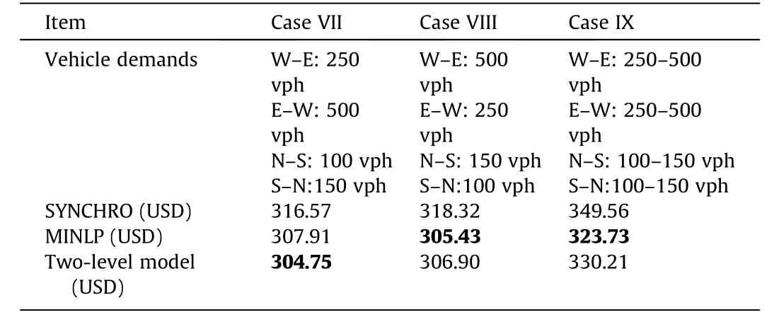
Table 6 Total cost from different methods under various demand levels in opposite directions.

Fig. 7. Improvement of model performance over SYNCHRO for Cases VII-IX.

The numerical experiments test of different methods in ten cycles range from 10 to 20 min based on the cycle length. The simulation period can be extended but doing so requires a significant longer computation time. The NOMAD solver may fail to find feasible solutions under high vehicle demand levels and short signal plan updating intervals(meaning a larger number of variables).The two-level model can generally ensure convergence, but the computation time also varies based on the aforementioned factors.Fig. 9 shows the number of iterations for different offset updating intervals for Case I. Usually, the program will converge within ten iterations for different cases. Similar patterns are found for other cases, which are omitted here.

4. Conclusions

This study developed a signal timing optimization and coordination framework in the CV environment that considers individual vehicle’s trajectories. The problem was first formulated in a centralized scheme as an MINLP accounting for the fixed cycle length constraint in order to optimize the phase durations and offsets in one mathematical program. The IDM was applied to estimate and predict the vehicle trajectories, considering a 100% penetration rate of CVs. Due to the complexity of the model, we decentralized the problem into two levels:an intersection level to generate optimal phase durations using the DP method the authors developed previously for each intersection, and a corridor level to update the optimal offsets for all the intersections. The two-level model reduces the complexity of the MINLP. In order to solve the twolevel model, we further developed a prediction-based solution technique that can solve the problem iteratively. We tested the proposed models and solution technique in a corridor containing five intersections through traffic simulation. The results from the MINLP and the two-level model both outperformed the signal optimization and coordination plan generated by SYNCHRO in terms of traffic delay and fuel consumption. This was tested using nine cases with different traffic volumes and vehicle types. The results also suggested that signal coordination may bring limited benefits to intersections with low traffic volume or to vehicles on minor streets. For future research, we will relax the assumption of a 100% CV penetration rate. This requires certain trajectory estimation techniques for non-CVs based on the sampled CV trajectories.Moreover, the proposed two-level method will be tested and validated using more data,such as real-world traffic volume and signal timing data.

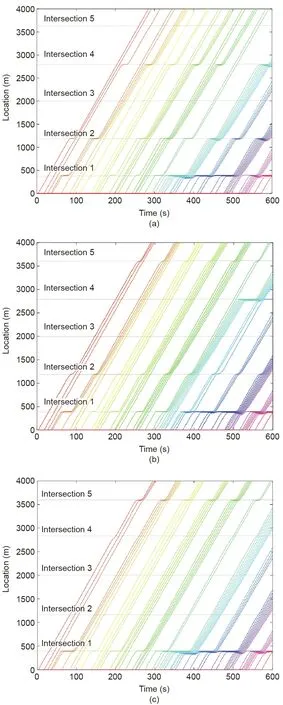
Fig. 8. Vehicle trajectories from different signal plans. (a) Trajectories from the SYNCHRO signal plan; (b) trajectories from the MINLP signal plan; (c) trajectories from the two-level model signal plan.

Fig.9. Convergence of the two-level model for Case I.(a)Offset updating in every 5 cycles; (b) offset updating in every 10 cycles.

Acknowledgements

The authors would like to thank the two anonymous reviewers for their insightful comments that helped improve the original version of this paper. This research is partially supported by the connect cities with smart transportation (C2SMART) Tier 1 University Transportation Center (funded by US Department of Transportation(USDOT))at the New York University via a grant to the University of Washington (69A3551747124).

Compliance with ethics guidelines

Wan Li and Xuegang Ban declare that they have no conflict of interest or financial conflicts to disclose.