GLOBAL WEAK SOLUTIONS FOR A NONLINEAR HYPERBOLIC SYSTEM*

Qingyou SUN (孙庆有) Yunguang LU (陆云光)†

K.K.Chen Institute for Advanced Studies, Hangzhou Normal University, Hangzhou 311121, China

E-mail : qysun@hznu.edu.cn; ylu2005@ustc.edu.cn

Christian KLINGENBERG

Department of Mathematics, Wuerzburg University, Wuerzburg 97070, Germany

E-mail : klingenberg@mathematik.vehi-wuerzburg.de

Key words global weak solutions; viscosity method; compensated compactness

1 Introduction

In this paper, we study the global solutions of the nonlinearly conservation system of three equations

with bounded initial data

Substituting the first equation in (1.1) into the second and the third, we have, for the smooth solution, the following equivalent system about the variables (ρ,u,s),

Let the matrix dF(U) be

Then three eigenvalues of (1.1) are

with corresponding three Riemann invariants

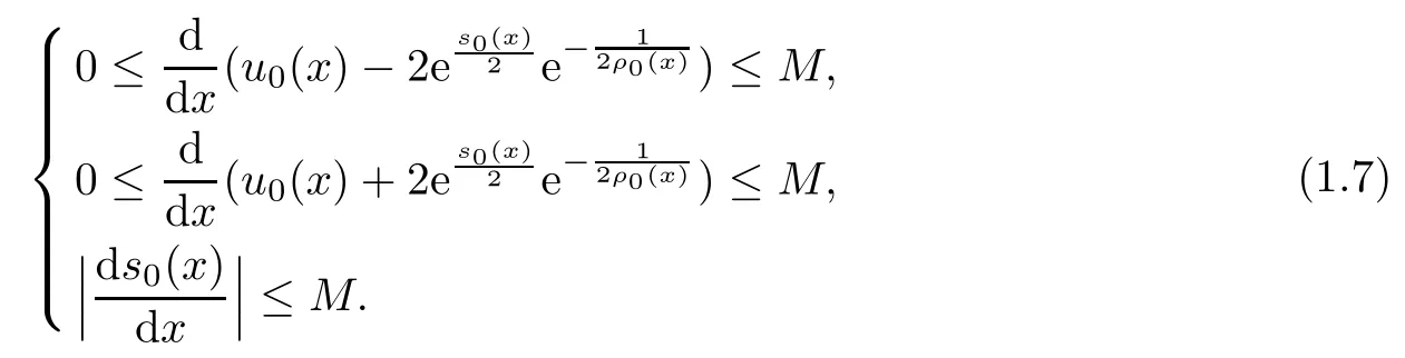
Based on the following condition (H), the existence of global smooth solution for the Cauchy problem (1.3) and (1.2) was first studied in [1]:

(H) ρ0(x),u0(x),s0(x) are bounded in C1(R), and there exists a positive constant M such that

However,there is a gap in the proof in[1]because the same estimates,like(1.7),on the solution(ρ(x,t),u(x,t),s(x,t)), do not ensure the boundedness of (ρ(x,t),u(x,t),s(x,t)).

In this paper, we shall repair this gap by assuming that the amplitude, of the first two Riemann invariants (w1(x,0),w2(x,0)) of system (1.1), is suitable small (see the condition(1.9) below), and weaken the condition (H).

Mainly we have the following result.

Theorem 1.1Let(ρ0(x),u0(x),s0(x)) be bounded,ρ0≥ 0,s0≥ 0. w1(x,0)and w2(x,0)are nondecreasing, and there exist constants c0,c1,c2,M such that

Then the Cauchy problem (1.1) and (1.2) has a generalized bounded solution (ρ(x,t),u(x,t),s(x,t)) satisfying that the first and the second Riemann invariants w1(x,t),w2(x,t) are nondecreasing andR|sx(x,t)|dx ≤M.

It is worthwhile to point out that a similar result on nonlinear system of three equations was obtained in[2],where the authors studied the global weak solution for the following system

where P(ρ,s)=e(γ−1)sργ.

This paper is organized as follows: In Section 2, we introduce a variant of the viscosity argument, and construct the approximated solutions of the Cauchy problem (1.1) and (1.2) by using the solutions of the parabolic system(2.1)with the initial data(2.2). Under the conditions in Theorem 1.1,we can easily obtain the necessary boundedness estimates(2.8),(2.9)and(2.10)on the approximated solutions where the bound M(δ,T) in(2.9) could tend to infinity as δ goes to zero or T goes to infinity. In Section 3, based on the estimates (2.9) and (2.10), we obtained the pointwise convergence of the viscosity solutions(ρε,δ(x,t),uε,δ(x,t),sε,δ(x,t)) by using the compensated compactness theory [3–13].

2 Viscosity Solutions

In this section we construct the approximated solutions of the Cauchy problem (1.1) and(1.2) by using the following parabolic systems

with initial data

where ε,δ are small positive constants, Gδis a mollifier. and (ρ0(x),u0(x),s0(x)) are given by(1.2). Thus wi(x,0),i=1,2,3, are smooth functions, and satisfy

where M is a positive constant being independent of δ and M(δ) is a constant, which could tend to infinity as δ tends to zero.

First, following the standard theory of semilinear parabolic systems, the local existence result of the Cauchy problem (2.1), (2.2) can be easily obtained by applying the contraction mapping principle to an integral representation for a solution.

Lemma 2.1Let wi(x,0),i=1,2,3, be bounded in C1space and satisfy (2.3) and (2.4).Then for any fixed ε>0,δ >0, the Cauchy problem (2.1) and (2.2) always has a local smooth solutionfor a small time τ, which depends only on the L∞norm of the initial data wi(x,0),i=1,2,3, and satisfies

Second, by using the maximum principle given in [14], we have the following a priori estimates on the solutions of the Cauchy problem (2.1) and (2.2).

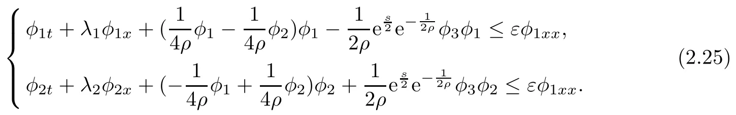
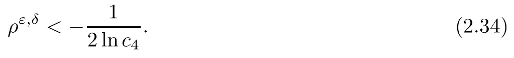
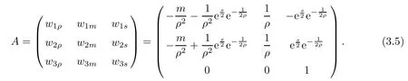
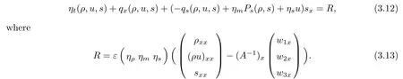
Lemma 2.2Let wi(x,0),i = 1,2,3 be bounded in C1space and satisfy (2.3) and (2.4).Moreover, suppose thatis a smooth solution of (2.1), (2.2) defined in a strip (−∞,∞)×[0,T]with 0

where the bound M(δ,T) could go to infinity as δ goes to zero or T goes to infinity.

ProofThe estimates in (2.8) can be obtained by using the maximum principle to (2.1),(2.2) and the condition (2.3) directly.

We differentiate (2.1) with respect to x and let wix= φi,i = 1,2,3; then we have the following parabolic system

In general, the maximum principle of the parabolic system (2.11) depends on the sign of the zeroth-order terms’s coefficientFortunately, since we only need to prove the nonnegativity of≥0, the sign ofcan be ignored. In fact,make a transformation

where L,c,N,β are positive constants and N is the upper bound of φion R × [0,T](N can be obtained by the local existence). The function Φ, as is easily seen, satisfies the equation

resulting from (2.11). Moreover

From (2.13), (2.14) and (2.15), we have

If (2.16) is violated at a point (x,t) ∈(−L,L)× (0,T), letbe the least upper bound of values of t at which Φ(x,t)>0, then by the continuity we see that Φ(x,t)=0, at some points

If we choose sufficiently large constants β,c such that

the equation (2.13) gives a conclusion contradicting (2.18). So (2.16) is proved. Therefore, for any point (x0,t0)∈ (−L,L)×(0,T),

which give the desired estimates φi≥ 0,i=1,2, if we let L in (2.20) go to infinity.

Since λ3=u,w3=s, the third equation in (2.11) is

To prove the left estimates in (2.9), we first calculate λiwj,i = 1,2,j = 1,2,3. By simple calculations, we have from the Riemann invariants given in (1.6)

Then the first and second equations in (2.11) are

By using the nonnegativity of φ1,φ2, we have from (2.24) that

Then we have from (2.25) that

By using the nonnegativity of X,Y again, we have from (2.27) that

From the conditions in (2.4), we have

Repeating the proof of Lemma 2.4 in [14], where λ=0 in our case,we can obtain by using the maximum principle to (2.28), (2.29) that

Finally using the same technique to estimate (2.8) in [15], we can prove (2.10) from (2.5), and so complete the proof of Lemma 2.2.

From the estimates (2.8) and (2.9), we have the following estimates about the functions(ρε,δ,uε,δ,sε,δ). First, from (2.8), we have

for a suitable constant c(δ), which could go to zero as δ goes to zero. Moreover,

which implies

Second, from (2.9), we have

Based on the a priori estimates given in (2.8) and (2.9) on the local solution, and the positive lower bound (2.33), we may extend the local time τ in Lemma 2.1 step by step to arbitrary large time T and obtain the following global existence of solution for the Cauchy problem(2.1)and (2.2).

Theorem 2.3Let wi(x,0),i=1,2,3 be bounded in C1space and satisfy(2.3)–(2.5),then the Cauchy problem(2.1)and(2.2)has a unique global smooth solution satisfying(2.8)–(2.10).

3 Proof of Theorem 1.1

In this section, we shall prove Theorem 1.1. First, based on the BV estimate (2.10)on the sequence of functions sε,δ, we have the following lemmas

Lemma 3.1For any constant c,are compact in

ProofSinceare bounded infrom(2.10),hence compact infor α ∈(1,2)by the Sobolev embedding theorem. Noticing thatare bounded in W−1,∞,we get the proof by Murat’s theorem [16]thatare compact in

From the third equation in (2.1), we have that

Second, we prove the pointwise convergence of sε,δ.

Lemma 3.2There exists a subsequence(still labelled)sε,δsuch that when ε goes to zero more fast than δ,

where s(x,t) is a bounded function, and Ω ⊂ R × R+is any bounded open set.

ProofUsing the results in Lemma 3.1, we may apply the div-curl lemma to the pairs of functions

We are going to complete the proof of Theorem 1.1 by proving the pointwise convergence of ρε,δand uε,δ.

Let the matrix A be

By simple calculations, the inversion of A is

We multiply (2.1) by A−1to get

Now we fix s as a constant, and consider the following system about the variables ρ,u:

A pair of smooth functions(η(ρ,u,s),q(ρ,u,s))is called a pair of entropy-entropy flux of system(3.8) if (η(ρ,u,s),q(ρ,u,s)) satisfies the additional system

or equivalently

Eliminating the q from (3.10), we have

For any smooth pair of entropy-entropy flux (η(ρ,u,s),q(ρ,u,s)), we multiply (ηρ(ρ,u,s),ηm(ρ,u,s),ηs(ρ,u,s)) to (3.7), where m= ρu, to obtain

By using the estimate (2.10), we have that (−qs(ρ,u,s)+ ηmPs(ρ,s)+ ηsu)sxis uniformly bounded in L1(R×R+), and hence compact infor α ∈ (1,2)by the Sobolev embedding theorem. If we choose ε to go zero much fast than δ, by using the estimates in (2.35), we have that R is compact inTherefore, we have the following Lemma:

Lemma 3.3For any fixed s, let (η(ρ,u,s),q(ρ,u,s)) be an arbitrary pair of smooth entropy-entropy flux of system (3.8). Then

Thus for fixed s, for smooth entropy-entropy flux pairs (ηi(ρ,u,s),qi(ρ,u,s)),i = 1,2, of system (3.8), the following measure equations or the communicate relations are satisfied

where ν(x,t)is the family of positive probability measures with respect to the viscosity solutions(ρε,δ,uε,δ,sε,δ) of the Cauchy problem (2.1) and (2.2).

Therefore by using the framework from the compensated compactness theory, given in [3–6], we may deduce that Young measures given in (3.15) are Dirac measures, and the pointwise convergence of ρε,δand uε,δ. Theorem 1.1 is proved.