Construction of Spatiotemporal-Coupling Optimal Low-Dimensional Dynamical Systems for Compressible Navier-Stokes Equations
2022-11-09 05:52QIJinWUChuijie
应用数学和力学 2022年10期
QI Jin,WU Chuijie
(1.Institute of Applied Physics and Computational Mathematics,Beijing 100088,P.R.China;2.School of Aeronautics and Astronautics,Dalian University of Technology,Dalian,Liaoning 116024,P.R.China)
Abstract:For the low-dimensional dynamical system model to study dynamics properties of Navier-Stokes equations,it is very important that the attraction domain of the low-dimensional model is the same as that of Navier-Stokes equations.However,to date,there is no universal approach to ensure this purpose for general problems.Herein,it is found that any low-dimensional model based on spatial bases,such as proper orthogonal decomposition bases,optimal spatial bases,and other classical spatial bases,is not predictable,i.e.,the error increases with the time evolution of the flow field.With the theoretical framework for building optimal dynamical systems and the new concept of spatiotemporal-coupling spectrum expansion,the low-dimensional model for compressible Navier-Stokes equations was constructed to approximate the numerical solution to large-eddy simulation equations,and the numerical results and novel time evolution of spatiotemporal-coupling bases were given.The entire field error is typically below 10-2%,and the average error at each grid point is below 10-8%.The spatiotemporal-coupling optimal low-dimensional dynamical systems can ensure that the attraction domain of the low-dimensional model is the same as that of Navier-Stokes equations.Therefore,characteristic dynamics properties of spatiotemporal-coupling optimal low-dimensional dynamical systems are the same as those of real flow.
Key words:spatiotemporal spectrum expansion;spatiotemporal-coupling optimal low-dimensional dynamical system;compressible Navier-Stokes equations;large-eddy simulation;quantitative comparison
1 Introduction and Overview
1.1 Research Background
For a long time,mathematicians and physicists have been concerned with the solution and research of PDEs(partial differential equations).However,except for a few simple cases,it is very difficult to solve the Navier-Stokes equations.For the general 3D flow problems,the existence and uniqueness of the theoretical solution have not been proven[1],and it is extremely difficult to study complex flows,such as turbulence.
In the long-term study of turbulence,organized large-scale structures have been found in seemingly disordered flow,i.e.,coherent structures,which are composed of vortices with different scales.These coherent structures play a decisive role in the generation and development of turbulence.The study of coherent structures and the establishment and analysis of turbulent low-dimensional dynamical systems are one of the key perspectives to understand the physical essence and law of turbulence.
From the perspective of dynamical system theory,the Navier-Stokes equations belong to an infinite dimensional dynamical system.To study the variation law of its solution with parameters,one of the more feasible methods is to study the nonlinear dynamic characteristics of its low-dimensional dynamical system(LDDS),that is,the dynamical system of infinite-dimensional PDEs is reduced to the finite low-dimensional dynamical system[2-3],i.e.,a set of ordinary differential equations,and the main characteristics of the original system are retained in the finite-dimensional system to the greatest extent.Therefore,for some infinite-dimensional dynamical systems of PDEs,the long-term behaviour and dynamic characteristics can be described and studied in finite-dimensional dynamical systems.This kind of nonlinear dynamic behaviour with the changes of characteristic parameters(including the Reynolds number,Mach number,etc.)plays an important role in the study of complex flows(including the occurrence,development and interaction of instability,turbulence,shock waves,etc.).
In recent years,many researchers[4-7]have given attention to the modelling and analysis of low-dimensional dynamical systems in turbulence research.Through the Galerkin projection of the Navier-Stokes equations onto a set of suitable bases functions,a low-dimensional dynamical system model consisting of ordinary differential equations with time-varying spectral coefficients was obtained.
1.2 The Construction Methods for Low-Dimensional Dynamical System Models
Dynamical system modelling methods can be divided into the following two categories according to the relationship with PDEs.
1.2.1 The Modelling Method Independent of PDEs
The Galerkin method[8]based on the Fourier decomposition and the local Taylor expansion[9]of flow fields are commonly used to build low-dimensional dynamical systems.The modelling method of energy stability analysis[10-11]was proposed by Lumley et al.,which extracts the flow structure with the largest part of the kinetic energy growth rate,constructs the bases,and then analyses the coherent structure of turbulence.
1.2.2 The Modelling Methods Related to PDEs
①The POD(proper orthogonal decomposition)methods
The essence of this method is to extract the orthogonal bases in the sense of least squares from the numerical simulation or experimental data objectively without prejudice and use the linear combination of fewer bases to approximate and describe the characteristics of the original database and physical process[12].Therefore,it is an efficient dimension reduction method.
The application of the POD method can be traced back to the work of Italian geometer Beltrami in 1873 and was first proposed by ref.[13].It is also called Karkunen-Loéve decomposition(in meteorology,it is called the principal component analysis method[14]).Hofmes and Lumley et al.[3,10,12,15]introduced the POD method to the study of turbulence for the first time.Through the Galerkin projection of Navier-Stokes equations on the POD bases,a set of low-dimensional models were obtained,and then,the flow characteristics were analysed.However,their lowdimensional models must be built on the known turbulence database,and there are serious problems in the satisfaction of incompressibility and boundary conditions.
It must be pointed out that the POD method has 3 limitations as follow.First,the method is limited to the form of the inner product optimal condition.When the essential characteristics of the system cannot be expressed with the inner product optimal conditions,the method cannot be used to analyse some key regions(including the generation of boundary vorticity flow,etc.)or accurately describe the important flow phenomena at a certain moment(including the dynamic characteristics of vortex breakdown,etc.).Second,due to the existence of projection errors,the low-dimensional dynamical system constructed with the POD method is not necessarily optimal.In the strict sense,this method is only a better means of data processing and analysis.Third,POD bases must be obtained from known databases and cannot be obtained directly from PDEs.
②The OLDDS(optimal low-dimensional dynamical system)theory
To further reduce the dimension and retain the flow field characteristics as much as possible,Wu and Shi[16-17]proposed the optimization theory for flow database analysis and low-dimensional dynamical systems,which is a more extensive new theory completely different from the POD method.The basic idea of the OLDDS theory is to determine theN-order optimal bases(OBs)to form theN-order intrinsic coordinate system with the methods of optimal control and functional analysis.In this way,theN-order optimal hyperplane derived from this intrinsic coordinate system can approach the exact solution to the infinite-dimensional dynamical system(infinitedimensional manifold),in the sense of the minimum norm at the parameter value of the studied system,in a wide range of parameters.
Since 1994,the OLDDS theory[18-23]has been further developed.The flow field structures of a 2D square cavity flow and a backstage step flow were studied,and the Lorenz OLDDS was established to analyse its nonlinear dynamic characteristics.Recently,based on the optimal functional of the minimum weighted residuals,the OLDDS model for the 3D incompressible Navier-Stokes equations[24]was obtained.For the first time,the authors applied the HWD(helical-wave decomposition)method to the modelling of OLDDS and proposed the generalized HWD-POD OLDDS method of coherent structures[21],and based on this method,the coherent structures of 3D channel turbulence and the characteristics of its dynamical system were studied.Furthermore,the optimal generalized helical-wave dynamical system of 3D backward-facing step flow was established[25],and the turbulent elements,i.e.,optimal GHWD(generalized helical-wave decomposition)vortices with spatial concentration and slow time-varying characteristics,were obtained.
Recently,the authors and their students developed an OLDDS modelling method for the 3D incompressible Navier-Stokes equations that satisfies both the arbitrary velocity boundary conditions and the incompressible conditions with the OLDDS modelling method,obtaining the OLDDS model for 3D square cylinder groups(including 1,2 and 3 square cylinders).Moreover,dynamical system analysis tools(such as the phase space orbit,the Poincaré section,the power spectrum,the Lyapunov exponent set analysis and the bifurcation analysis)were used to analyse the complex dynamical system characteristics of 3D square cylinder groups[26-28].It is found that the dynamic characteristics of the wake of a square cylinder are limit cycles.On the other hand,the fluctuating velocity characteristics of the wake of 2 square cylinders are more complicated limit cycles,and the behaviour of the fluctuating OLDDS on its bifurcation diagram is similar to that of period doubling bifurcation,which indicates that more complex dynamic behaviour begins to appear.Based on the dynamical system analysis of OLDDS models(with truncationN=10)of the 3 square cylinder wakes,it is found that the Poincaré section of the wake of 3 square cylinders exhibits chaotic trajectories and broadband power spectra.Through the analysis of its Lyapunov exponent set,it is found that 6 of its 10 Lyapunov exponents are positive,1 is 0 and 3 are negative,which indicates that the OLDDS behaviour of the wake of 3 square cylinders is chaotic.Thus,it can be seen that in the heat exchanger application,the complexity of the wake can be enhanced by multi-component flow,to promote fluid mixing and improve heat exchange efficiency.It also can be seen that the OLDDS method provides a feasible method to solve the key problems in turbulence research.
It is very difficult to model and analyse the low-dimensional dynamical system of compressible Navier-Stokes equations,there are almost no reports addressing this aspect.The outline of the rest of this paper is as follows.The research objectives are introduced in section 2.The construction theory of spatiotemporal-coupling optimal lowdimensional dynamical system(SCOLDDS)for the general problem is presented in section 3.The construction theory of SCOLDDS for the compressible Navier-Stokes equations is presented in section 4.Applications of SCOLDDS are shown in section 5.Concluding remarks are made in section 6.
2 Research Objectives
To analyse the low-dimensional dynamical system of compressible Navier-Stokes equations,the most important thing is to obtain a suitable low-dimensional dynamical system model which can reflect the characteristics of the original system as much as possible.The modelling method of OLDDS shall satisfy the following 2 conditions:
①Various boundary conditions.However,for complex problems,the usual homogenization cannot be used because it turns one complex problem into another equally complex one.In the Galerkin spectrum method,the basis function that satisfies the boundary conditions is actually a sufficient condition,and it can only be used for periodic boundary conditions and nonslip velocity boundary conditions.Therefore,for the general problem,when the Galerkin spectrum method is used to model the OLDDS and the basis function is still used to satisfy the boundary conditions,the following 2 problems will be encountered:first,for given velocity boundary conditions(such as inflow boundary conditions),how to solve the problem of “1 to many”,i.e.,how to assign a velocity boundary condition toNoptimal bases;second,how to solve the strong solution boundary condition proposed by unsteady boundary conditions(such as the time-varying outflow boundary condition),given that any spatial basis function can only satisfy the weak solution form of the unsteady boundary condition,that is,it can only satisfy the time-averaging unsteady boundary condition.
②Quantitative comparison to the numerical simulation results of computational fluid dynamics(CFD).The most substantial limitation of the traditional low-dimensional dynamical system modelling method is that,it cannot establish the low-dimensional dynamical system model based on an accurate quantitative comparison with highdimensional CFD results because only when the dimension of classical spectrum expansion is very large(hundreds of thousands of dimensions),can it meet the requirement of accurate quantitative comparison.However,the calculation of long-term characteristics of turbulence with high-dimensional dynamical system models is very cumbersome.Therefore,the traditional dynamical system research adopts a very low-dimensional dynamical system model(such as the 3D Lorenz model),but the essential dynamical system characteristics of the low-dimensional model are likely to be completely different from those of the real turbulence(that is,they are in different regions of the functional space).
Therefore,it is necessary to extend the OLDDS modelling theory.In this paper,a SCOLDDS modelling method was proposed to obtain a SCOLDDS model for compressible Navier-Stokes equations that satisfies various complex geometrical and physical boundary conditions and can be quantitatively compared with high-dimensional numerical simulation results.
The SCOLDDS of turbulence established based on an accurate quantitative comparison is not only in the same region of functional space as the real turbulence dynamical system but its SCOBs(spatiotemporal-coupling optimal bases)are also coherent structures,and the intrinsic optimal bases are very low-dimensional(such as the 3rd-order SCOBs used in this study);therefore,the very low-dimensional SCOLDDS can be obtained,which can greatly reduce the amount of calculation in the study of long-term characteristics of turbulent dynamical systems.
3 The Construction Theory of SCOLDDS for General Problem
3.1 The Basic Idea and the Essential Innovation of Optimal Bases
The basic idea of the OLDDS theory for PDEs is shown in fig.1;i.e.,with the methods of optimal control and functional analysis,theN-order intrinsic coordinate system composed ofN-order optimal bases is obtained so that theN-order optimal hyperplane constructed from theN-order intrinsic coordinate system can approach the exact solution to the infinite-dimensional dynamical system(infinite-dimensional manifold)well in the sense of the minimum norm at the parameter value of the studied system and in a wide range of parameters.
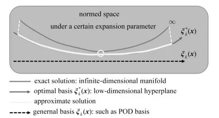
Fig.1 The basic idea of the OLDDS theory
The most substantial difference between theN-order optimal bases and the traditional spectral expansion is that in the spectral expansionof system variablesu(x,t),optimal basesare not given in advance,and theN-order optimal bases that depend on the given differential equations and initial and boundary conditions are obtained with the optimal control method under the condition of satisfying the quantitative comparison,the given optimal functional and other constraints.The low-dimensional dynamical system model based on the optimal basesis an OLDDS.
The starting point of the theory of low-dimensional dynamical systems for PDEs is spectral expansion:

whereuRis the remainder,Nis the order of spectral expansion,ξkare basis functions,also called spectral functions.For classical spectral expansion,ξkare known spatial bases,i.e.,ξk=ξk(x).For optimal bases,are not given in advance.TheN-order optimal bases that depend on the given differential equations and initial and boundary conditions are obtained with the optimal control method under the condition of satisfying the given optimal function and other constraints.
The essential innovation of the theory of SCOLDDS proposed in this paper is that the basis functions areNorder optimal basesrelated to physical problems,and if the SCOBs are used to represent the spatiotemporalcoupling characteristics of the system,they are SCOBsor if the time-averaged characteristic of the system is represented by the spatial optimal bases,they are optimal spatial bases.
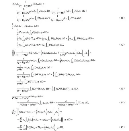
Because the snapshot POD bases must satisfy the ergodic condition of each state,periodTcannot be too small,so the real-time spatiotemporal-coupling POD bases cannot be obtained.On the other hand,because all spatiotemporal flow data must be used to find the POD bases,whenTis very large,the amount of calculation of POD will be to high,so the full time-space POD bases cannot be obtained.Therefore,it is impossible to obtain the SCOLDDS model based on POD bases.
3.2 The Mathematical Problem and the Construction of Low-Dimensional Models
3.2.1 The Mathematical Problem
For the initial boundary value problem of general PDEs,whose governing equations,initial conditions and boundary conditions are as follow:

3.2.2 The Construction of Low-Dimensional Models

3.2.3 The Optimal Problem of Obtaining the Optimal Basis

4 The Construction Theory of SCOLDDS for Compressible Navier-Stokes Equations
4.1 Compressible Navier-Stokes Equations
In Cartesian coordinates,the dimensionless 3D unsteady compressible Navier-Stokes equations[32](including the continuity equation,the momentum equation,the energy equation,the state equation,and the initial and boundary conditions,with the exception of hypersonic flow,i.e.,regardless of the ionizing radiation of a fluid)are considered:


4.2 Spatiotemporal-Coupling Low-Dimensional Dynamical Systems for Compressible
Navier-Stokes Equations and Numerical Realization of Boundary Conditions
4.2.1 Spatiotemporal-Coupling Low-Dimensional Dynamical Systems for Compressible Navier-Stokes Equations
The SCOLDDS modelling theory in section 3 are applied to the compressible Navier-Stokes equations to derive the SCOLDDS equations.

Therefore,the Galerkin projection expression of the energy equation on arbitrary temperature basis ηris obtained:
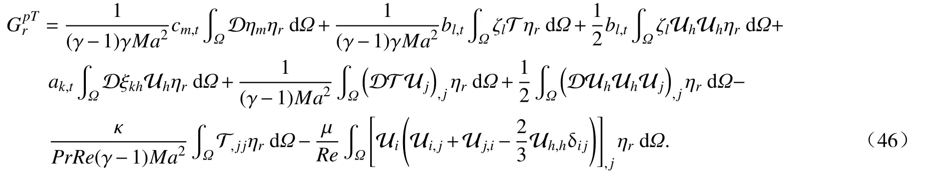
To summarize,the Galerkin projection equations of the following compressible Navier-Stokes equations are obtained:
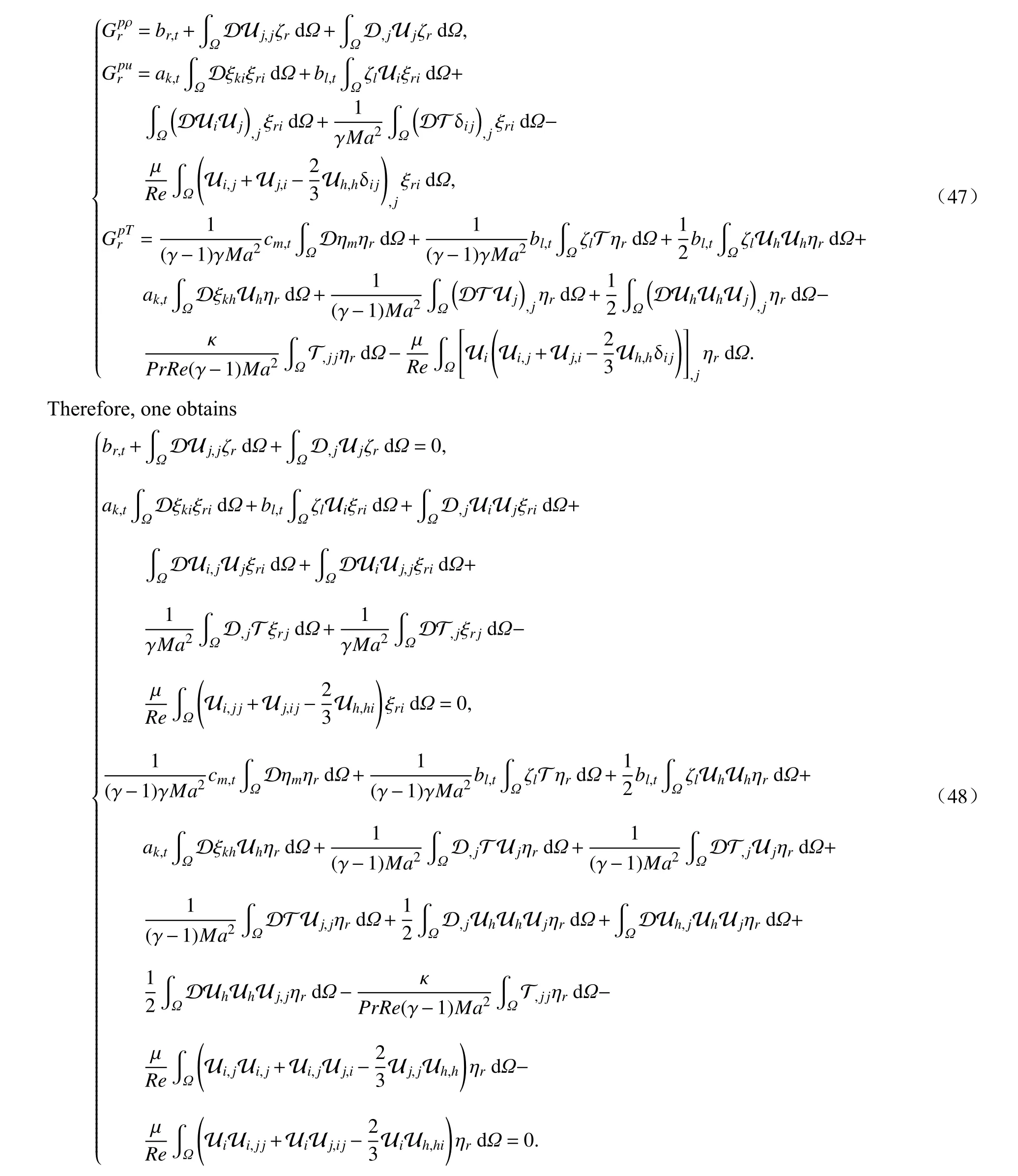
From this one obtains SCOLDDS equations eq.(49)for compressible Navier-Stokes equations:

where the coefficients are shown in eq.(51).The initial conditions are as follow:

4.2.2 The Numerical Realization of Boundary Conditions
Two methods are used to satisfy the boundary conditions,simultaneously,i.e.:
1)The optimal bases satisfying the boundary conditions are obtained with the optimal control method.
2)Boundary conditions F∂Ωare further satisfied in the physical space in solution of the dynamical system equations.Next,the boundary conditions of velocityuare taken as an example.
①Free-slip boundary conditions
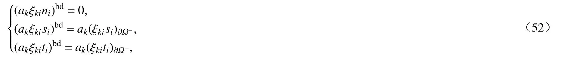
where superscript“bd”represents the boundary mesh,and subscript ∂Ω-represents a layer of mesh near the boundary.
②Nonslip boundary conditions
③Inflow boundary conditions

whereubiis the inlet velocity distribution function.
④Continuous outflow boundary condition

⑤Periodic boundary conditions

⑥For the compressible Navier-Stokes equations,the density boundary condition and the temperature boundary condition should also be satisfied.Specific methods for temperature and density are similar to the relevant parts of the above velocity boundary conditions and will not be repeated here.
4.3 The Optimal Functional of SCOLDDS for Compressible Navier-Stokes Equations
4.3.1 The Optimal Functional that Approximates Initial ConditionJand Its Gradient Equation
The optimal objective functional approximating the initial condition is

whereui(0),ρ(0),T(0)are the known initial values.
The following gradient equation can be obtained by finding the variation in eq.(57)and making the variation zero:

The conjugate gradient numerical optimization algorithm(see appendix A)is used to solve eq.(58).
4.3.2 The Multi-Scale Global Optimization Method
Model equation eq.(17)of the OLDDS obtained with the variational method is only the local extremum of generalized optimal objective functional eq.(18)in functional space BN,but we hope to obtain the global optimal bases in whole space BN.However,according to the fundamental theorem of global optimization:in general,one cannot obtain the global optimal solution unless an infinite number of searches are carried out,in practical calculations,the final convergence result depends on the selection of iterative initial basis(hereinafter referred to as initial bases)is near the global minimum ofJg,the final convergence results are the global optimal bases;otherwise,it can only converge to the local extreme point or even a saddle point ofJg.
Here,a multi-scale global optimization method is proposed to find the approximate global optimal solution.Based on the idea of coarse graining,the global optimal value is quickly located by smoothing the local extreme points.Suppose that value distributionJgof the generalized optimal objective functional corresponding to the exact solution to eq.(2)in space BNis shown as the red curve in fig.2.Then,to find global optimal valueA,the following process of the double-scale global optimization method can be implemented,as follows.
1)Coarse graining:a coarse numerical scheme or grid is used to numerically simulate the equation,a set of coarse databases is obtained.The change in generalized optimal objective functionalJg*based on the coarse database in space BNis shown by the green curve in fig.2.Coarsening makes the local extremum smooth and it can be regarded as a convex domain.
2)POD analysis:POD bases are extracted from the coarse database,and since POD bases are optimal for the database,the POD basis is located at pointBin fig.2.
3)Multi-scale computing:the POD basis extracted in step 2)is processed by interpolation to obtain a set of precise bases.Let the blue curve in fig.2 represent the value ofJg**of the generalized optimal functional in space BNcalculated in the fine grids.Then,the precise bases are located at pointCin fig.2.
4)Numerical optimization:with the precise bases obtained in step 3)as initial basisthe numerical optimization is carried out by substituting it into OLDDS model eq.(17),final convergence resultis located at pointDin fig.2,and then,can be considered as the approximate global optimal basis.database is only used to extract initial basisand no longer used in the following optimization process.

Fig.2 Schematic diagram of the double-scale global optimization method
According to the idea of double-scale global optimization,it can also be extended to additional multiple scales to obtain more accurate results.It should be emphasized that although the coarse database is used in this method,the
4.4 The Solution Procedure
Nrandom bases or POD bases of velocity,density and temperature can be used as the 1st,2nd and 3rd initial iteration bases ofrespectively.
1)Initialization:
(a)When the random bases are used as the initial iteration bases,the random number generator is used to generate the initial iteration random bases.When the POD bases are used as the initial iteration bases,the CFD/LES method is used to calculate the flow field of the 1st 500 CFD/LES time steps( Δt),and each flow field is taken for every 10 CFD/LES time steps,then,50 time sections of the flow field are obtained.From these 50 flow field data,50 POD bases are obtained with the snapshot POD method,and the 1stNPOD basesare taken as the initial iteration bases.
(b)With the optimization method which approximates the initial conditions in sectionandare obtained,and they are orthogonalized and normalized with the Grand-Schmidt method[36].Sett=0.
2)Lett=t+MΔt,whereMis the number of intervals of CFD/LES time steps.
3)Use the CFD/LES method to obtain the initial field of the dynamical system used in eq.(57)att=t+MΔt.
4)With the initial iteration bases and the optimization method which approximates the initial conditions in sectionare obtained,and they are orthogonalized and normalized with the Grand-Schmidt method[36].
5)By application of the initial conditions,eq.(50)is used to solve the SCOLDDS eq.(49)to obtainak(t),bk(t)andck(t).The boundary conditions must be satisfied in the 4 steps of the 4th-order Runge-Kutta method,and the illconditioned equation AFD method is used to preprocess the coupled equations.
6)Calculation of the physical quantities of the compressible flow field:
7)Return to step 2)until the calculation is completed.
5 Applications of the Construction Theory of SCOLDDS for Compressible Navier-Stokes Equations
In this section,since the flow fields of SCOLDDS and of compressible Navier-Stokes equations are very similar to each other,to save space the legends of flow field nephograms are not shown.
5.1 Definitions of Relative Errors of Flow Field Variables and Proportions of Each Order in the Whole Field
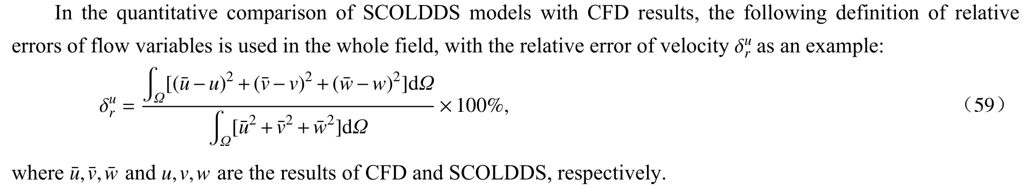
①Relative errors of flow variables in the whole field
②Proportions of flow variables of each order in the whole field
In order to understand the contribution of each order of flow variables to the total flow of the SCOLDDS,eq.(60)is used to calculate their proportions,as is shown below.Take velocity proportionas an example:

where |uk|,|vk|,|wk| are the absolute values of each component of the velocity field(such as|uk|=|akξk|,kdoes not sum up),and |u|,|v|,|w| are the absolute values of the velocity field(such as |u|=|akξk|),obtained with the SCOLDDS method,respectively.
5.2 The 3D Compressible Laminar Backward-Facing Step Flow
With this example,we will try to find the answers to following questions:
①How can the solutions to low-dimensional dynamical systems be quantitatively compariable with CFD results?
②What is the accuracy of the quantitative comparison between the results of SCOLDDS and CFD?
③What is the spatiotemporal evolution of SCOBs with the development of the flow field?
5.2.1 Research Problem
The dimensionless parameters of the 3D compressible laminar backward-facing step flow(fig.3)areRe=The finite volume method is used to solve the 3D unsteady compressible Navier-Stokes equations.Orthogonal meshes with equal spacings are used,Mx×My×Mz=85×41×41,(Δx,Δy,Δz)=(2.0,1.0,1.0)m,Δt=0.1 s.
The lower part of the left boundary is a nonslip backward-facing step,the upper part of the left boundary is an inflow boundary,the right boundary is a continuous outflow boundary,and the surrounding are nonslip solid wall boundaries.The height of the backward-facing step ish=20 m.The inflow velocity and density at the backwardfacing step of the left boundary areu0=(u0,v0,w0)=(0.56,0.0,0.0)m/s and ρ0=1.0 kg/m2,respectively,µ=
0.01 Pa·s.

Fig.3 The 3D sketch map of the compressible laminar backward-facing step flow
The SCOBs with truncationN=3 are used to construct the SCOLDDS model for compressible Navier-Stokes equations,and their solutions are compared with CFD results quantitatively in real time.
5.2.2 Numerical Experiments Predictability on the Low-Dimensional Dynamical System Models
In order to understand why the SCOBs are the key to obtaining the SCOLDDS,which ensures that the approximate solution to the SCOLDDS is in the attraction domain of the numerical solution of CFD(and the infinite-dimensional Navier-Stokes equations),a set of numerical experiments is conducted on the predictability of low-dimensional dynamical system models based on spatial bases and SCOBs with 3D compressible laminar backstage step flow.In the numerical experiments the velocity errors of various low-dimensional dynamical system models(such as POD bases,POD bases with a time interval,spatial optimal bases,SCOBs with random initial bases or POD initial bases)are shown in fig.4.
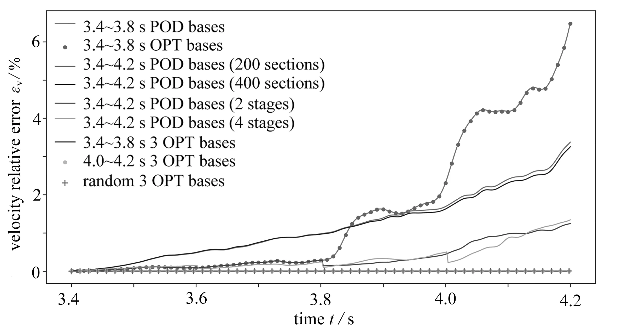
Fig.4 Comparison of the evolution curves of the velocity errors with time in the whole field of low-dimensional dynamical system models constructed by POD bases,POD bases with a time interval,spatial optimal bases,SCOBs with random initial bases or POD initial bases
In the following numerical experiments,the low-dimensional dynamical system models are constructed with POD bases,POD bases with a time interval,spatial optimal bases,SCOBs with random initial bases or POD initial bases,and the entire field's velocity errors of each approximate flow field are calculated by eq.(59).Four groups of test cases are studied.
1)Low-dimensional dynamical system models based on POD bases and SCOBs obtained in the period of 3.4 ~3.8s
①In the period of 3.4 ~3.8 s,200 snapshot POD bases are constructed,and then,the 1st 30 POD bases are used to obtain the low-dimensional dynamical system model through the Galerkin projection,and the approximate flow field of 3.4 ~4.2 s is obtained with the model.
②In the period of 3.4 ~3.8 s,the 3rd order spatial optimal bases are constructed;the low-dimensional dynamical system model is obtained through the Galerkin projection,and the approximate flow field of 3.4 ~4.2 s is obtained with the model.
2)Low-dimensional dynamical system models based on POD bases and SCOBs obtained in the period of 3.4 ~4.2 s
①In the period of 3.4 ~4.2 s,200 snapshot POD bases are constructed;the 1st 30 POD bases are then used to obtain the low-dimensional dynamical system model through the Galerkin projection,and the approximate flow field of 3.4 ~4.2 s is obtained with the model.
②In the period of 3.4 ~4.2 s,400 snapshot POD bases are constructed;the 1st 30 POD bases are then used to obtain the low-dimensional dynamical system model through the Galerkin projection,and the approximate flow field of 3.4 ~4.2 s is obtained by using the model.
3)Low-dimensional dynamical system models based on POD bases and SCOBs obtained in the multiple short periods
①In the periods of 3.4 ~3.8 s and 3.8 ~4.2 s,200 snapshot POD bases are constructed for each period;the 1st 30 POD bases are then used to obtain the low-dimensional dynamical system model through the Galerkin projection for each period,and the approximate flow field of 3.4 ~4.2 s is obtained with this 2-time-interval model.
②In the periods of 3.4 ~3.6 s,3.6 ~3.8 s,3.8 ~4.0 s and 4.0 ~4.2 s,200 snapshot POD bases are constructed for each period;the 1st 30 POD bases are then used to obtain the low-dimensional dynamical system model through the Galerkin projection for each period,and the approximate flow field of 3.4 ~4.2 s is obtained with this 4-timeinterval model.
4)Low-dimensional dynamical system models based on SCOBs
①In the period of 3.4 ~3.8 s,3.8 ~4.0 s and 4.0 ~4.2 s,3rd-order SCOBs with 3rd-order POD bases as initial bases are constructed.
②Third-order SCOBs with 3rd-order random initial bases are constructed;the low-dimensional dynamical system model is obtained through the Galerkin projection,and the approximate flow field of 3.4 ~4.2 s is obtained with these models.
From fig.4,it can be seen that:
(a)The dynamical system model based on spatial bases(including POD bases and spatial optimal bases)has fewer errors in the period of generating these bases,but the error becomes continually larger in the following time.Therefore,the low-dimensional dynamical system model based on spatial bases(including POD bases and spatial optimal bases)is not predictable.
(b)The error of the low-dimensional dynamical system model built on spatial bases constructed with a set of shorten period of data is smaller than that of with a set of longer period of data.
(c)The low-dimensional dynamical system model built on the SCOBs with random initial bases or POD initial bases can accurately approximate the CFD results,and the interval of solving SCOBs is not limited by the constrans of ergodic condition of each state in the snapshot-POD,and which can be from each CFD time step( dt)to any CFD time steps.At the same time,because the calculation of seeking the SCOBs does not rely on big flow field data,and its optimization convergence is very fast,the SCOLDDS model can be built efficiently and flexibly.
Therefore,one can arrive the conclusion that only with SCOBs,the accurate quantitative comparison between solutions of the SCOLDDS and the CFD of compressible Navier-Stokes equations is possible.
5.2.3 Results of Construction of SCOLDDS for Compressible Navier-Stokes Equations With 3D Compressible Laminar Backward-Facing Step Flow
①Time evolution curves of errors of compressible SCOLDDS models
It can be seen from fig.5 that at the beginning,because the initial iteration bases of velocity,density and temperature are the 3rd-order POD bases,the errors of flow field variables are large and then decrease rapidly during the solution SCOBs in the initial short time(N=3,Re=1 120,Ma=0.748 331 48,Pr=0.72).Second,the whole field error of the approximate flow field of the compressible SCOLDDS is kept below 0.01%,which shows that the average error at each point is kept below 0.01%/(85×41×41)=7×10-8%.
②Time evolution of the flow field:CFD vs.OLDDS
From fig.6,one can see the time evolution of the numerical solution with the finite volume method of Navier-Stokes equations and the approximate optimal solution of the 3rd-order SCOLDDS.The initial error is still obvious even after the optimal optimization because the POD bases are used as the initial iteration bases.However,after several optimal optimization processes,the approximate optimal solution of the 3rd-order SCOLDDS is very close to the numerical solution of CFD.

Fig.5 Time evolution curves of errors of velocity,density and temperature

Fig.6 Comparison of time evolution of flow fields of CFD and OLDDS,from left to right,t=100 s,300 s,5 000 s,9 990 s:(a)velocity field u;(b)velocity field v;(c)velocity field w;(d)density field ρ;(e)temperature field T
Therefore,the modelling method of SCOLDDS can obtain a high-precision approximate solution compared with the numerical solution of CFD and ensure that the optimal solution of the SCOLDDS with truncationN=3 is within the attraction domain of the numerical solution of the high-dimensional CFD(and with the infinitedimensional Navier-Stokes equations).Through analysis of the characteristics of the SCOLDDS with truncationN=3of the laminar backward-facing step,the exact dynamical system characteristics of the Navier-Stokes equations can be obtained.
③Time evolution curves of coefficients of SCOBs
It can be seen from fig.7 that,first,the coefficients of the 1st-order spatiotemporal-coupling velocity optimal basis ξ,density optimal basis ζ and temperature optimal basis η are one-order-magnitude larger than those of the 2nd- and the 3rd-order SCOBs.Therefore,the 1st-order SCOBs are dominant.Second,the coefficients of the 1storder SCOBs have a lower evolution frequency with time,while the coefficients of the 2nd-order and the 3rd-order SCOBs have higher evolution frequencies with time.
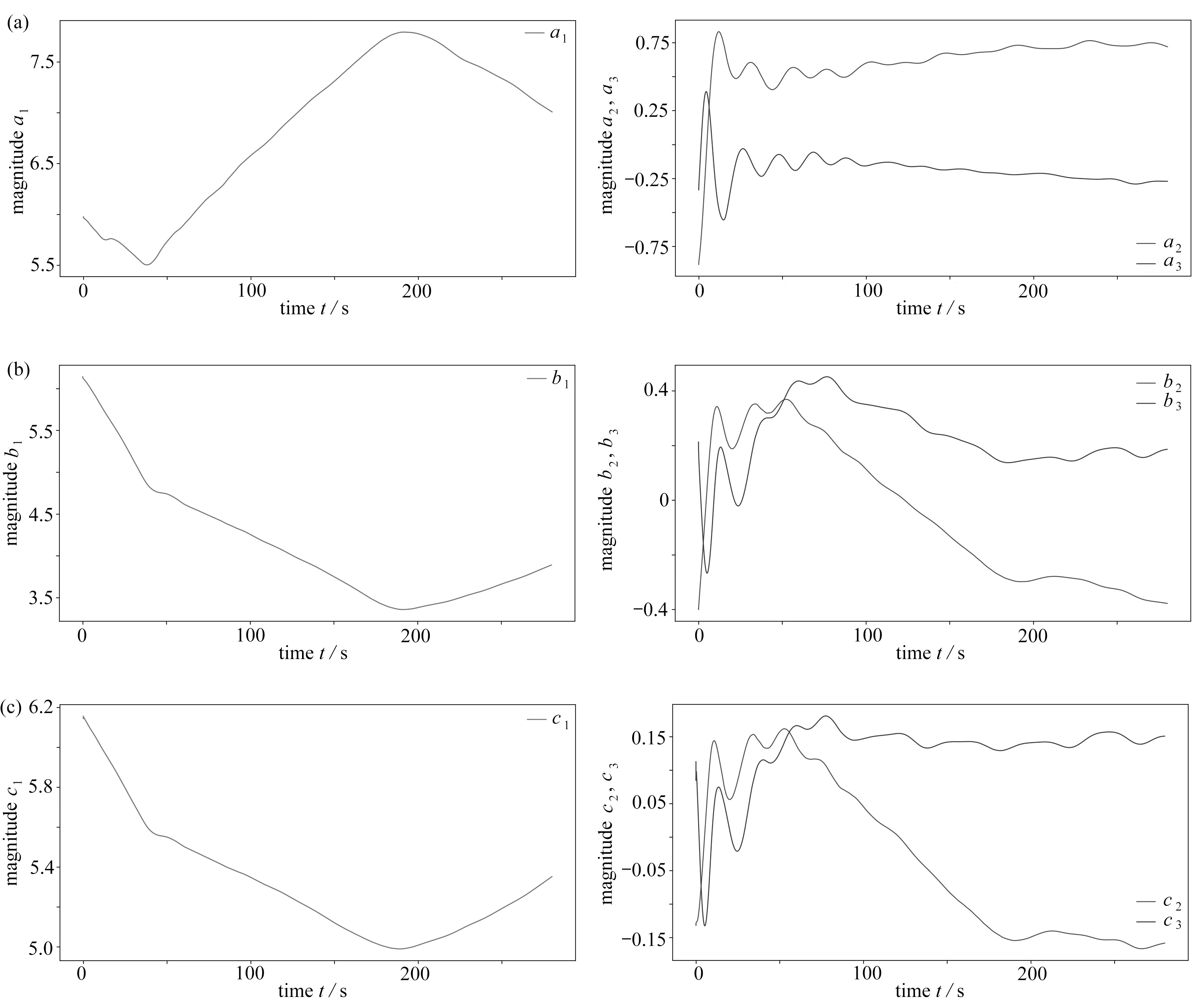
Fig.7 Time evolution curves of coefficients of velocity basis ξ,density basis ζ and temperature basisη
④Time evolution of spatiotemporal-coupling optimal velocity basis ξ,density basis ζ and temperature basisη
It can be seen from fig.8 that,for the laminar backward-facing step flow,the 1st-order spatiotemporal-coupling optimal velocity basis ξu,density basis ζ and temperature basis η dominate the time evolution of the flow field,and all evolve with the development of the flow,but their 2nd- and 3rd-order optimal bases basically do not evolve with time.However,the 1st-,2nd- and 3rd-order bases of velocity bases ξvand ξw,which are not dominant in the flow field,have obvious evolution with time.This may be because the 1st-order spatiotemporal-coupling optimal velocity bases ξvand ξw,which are not dominant in the flow field,have weak control over their 2nd- and 3rd-order SCOBs,the latter 2 can evolve synchronously with the development of the flow.
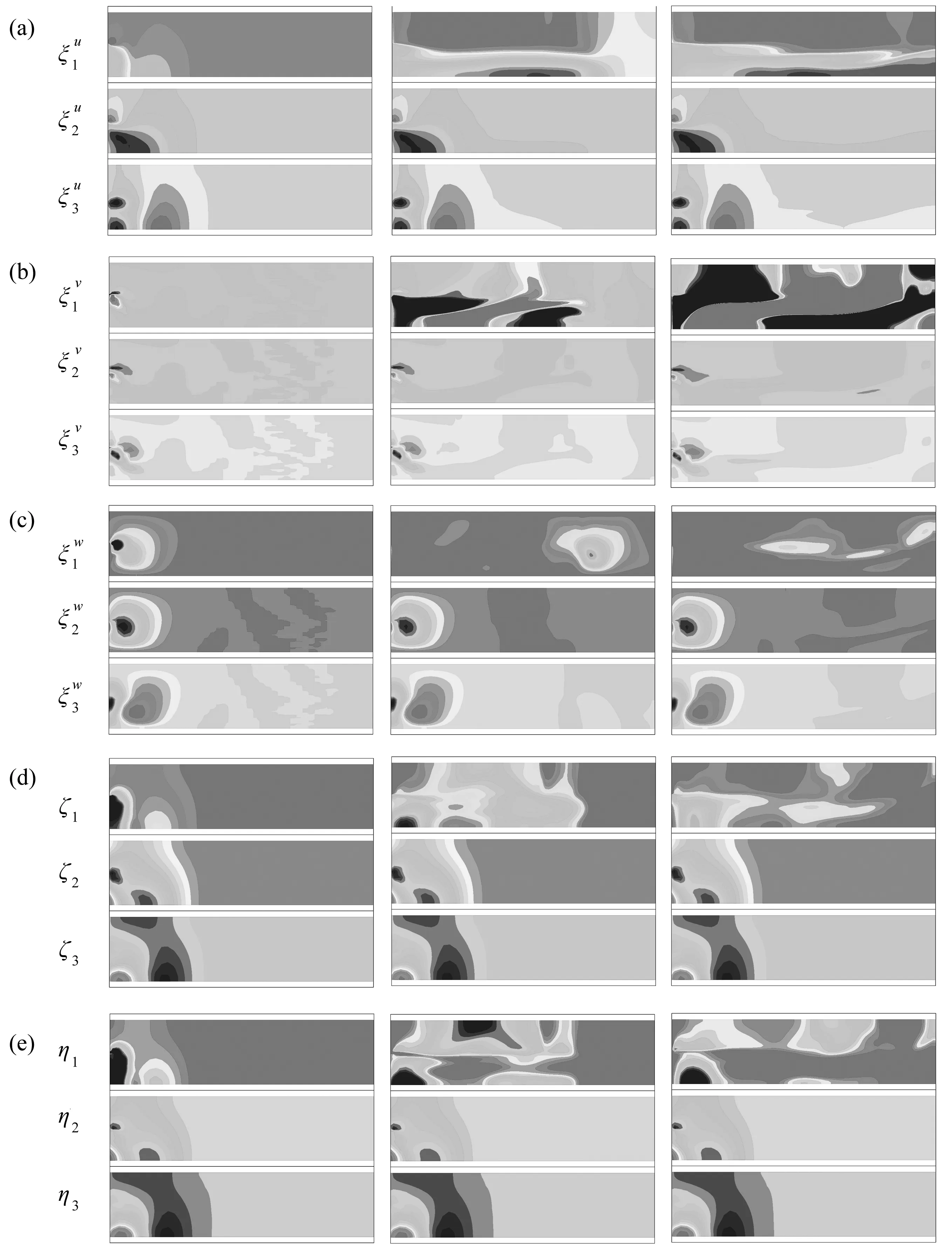
Fig.8 Time evolution of spatiotemporal-coupling optimal velocity basis ξ,density basis ζ and temperature basis η:from left to right,t=100 s,5 000 s,9 990 s
Through the observation of figs.7 and 8,one can draw the following conclusion:it is SCOBs that make SCOLDDS compare with CFD rigorously in numerical solution.
5.3 The 3D Compressible Turbulent Straight Jet
In this example,the answers to following questions will be found:
①Can the solutions of low-dimensional dynamical systems of compressible Navier-Stokes equations be quantitatively comparable with those of the large-eddy simulation(LES)of turbulent results?
②How is the accuracy of quantitative comparison between the results of SCOLDDS and LES?
③How is the importance of each order of decomposition,i.e.,how are the proportions(eq.(60))of each order of approximate flow variables in the turbulent jet flow with truncationN=3 and 5,respectively?
5.3.1 Research Problem
The dimensionless parameters of the 3D compressible turbulent straight jet flow(fig.9)areRe=Ma= 0.423 451 80,Pr= 0.72.

Fig.9 The 3D sketch map of the compressible turbulent straight jet flow
An LES method[37]based on the Favre filter[38-39]and Smagorinsky subgrid model[40],where Smagorinsky constantCs=0.1,is used to solve the 3D unsteady compressible LES equations.Orthogonal meshes with equal spacings are used,Mx×My×Mz=105×61×61,(Δx,Δy,Δz)=(1.5,1.0,1.0)m,Δt=0.000 58 s.
The diameter of the turbulent straight jet at the centre(y=z=31 m)of theyOzplane on the left boundary is Φjet=6 m,its inflow velocity isujet=(ujet,vjet,wjet)=(2.0,0.0,0.0)m/s,and its inflow density isρjet=0.627 59 kg/m3,µ=0.000 018 1 Pa·s.The inflow velocity and inflow density in the non-jet area on the left boundary areu0=(u0,v0,w0)=(0.3,0.0,0.0)m/s and ρ0=1.161 03 kg/m3,respectively,µ=0.000 018 1 Pa·s.The right boundary is a continuous outflow boundary,and the surrounding are nonslip solid wall boundaries.
The LES code is combined with the SCOLDDS modelling theory of 3D compressible Navier-Stokes equations to develop a 3D compressible turbulent LES and SCOLDDS modelling toolkit CLOT3D(compressible LES and SCOLDDS tools of 3D compressible Navier-Stokes equations).With this software package,the LES numerical solution of the turbulent straight jet is obtained,which is compared with the SCOLDDS model of compressible Navier-Stokes equations(using SCOBs with truncationN=3 and 5,respectively).
5.3.2 The SCOLDDS of the SCOBs With TruncationN=3
①Time evolution curves of errors of compressible SCOLDDS models
From fig.10,one can see that,given the turbulent straight jet flow,the time evolution of the velocity error is always very violent,but the whole field error is not large,basically below 0.006%.Since the whole field errors of density and temperature are very small(less than 0.001%),their time evolution process cannot be seen in the figure(Re=416 081.77,Ma=0.423 451 80,Pr=0.72,the same below).Second,because the velocity error of the approximate flow field of the compressible SCOLDDS is kept below 0.006% in the whole field,the average velocity error at each point is kept below 0.006%/(105×61×61)=1.5×10-8%.
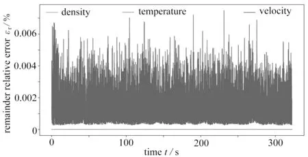
Fig.10 Time evolution curves of errors of velocity,density and temperature
②Time evolution of the flow field:LES ~ SCOLDDS
It can be seen from fig.11 that,for the first time,with the SCOLDDS model(N=3)for the compressible 3D Navier-Stokes equations can very accurately obtain the numerical results given by the LES method,and from the initial moment,the approximate optimal solution of the SCOLDDS with truncationN=3 can quickly approach the numerical solution of LES.

Fig.11 Comparison of time evolution of turbulent flow fields between the LES and the SCOLDDS,from left to right,t=100 s,5 000 s,16 670 s:(a)velocity field u;(b)velocity field v;(c)velocity field w;(d)density field ρ;(e)temperature field T
Therefore,a high-precision approximate solution can be obtained with the SCOLDDS modelling method,which guarantees for the first time that the optimal solution of the SCOLDDS has the same attraction domain as the numerical solution of the complex turbulent LES.Through analysis of the characteristics of SCOLDDS of the turbulent straight straight jet flow,the accurate characteristics of the turbulent dynamical system of the LES equations for the turbulent straight jet flow can be obtained.
③Time evolution curves of the proportion of each order of approximate flow variables(see eq.(60))
It can be seen from fig.12 that,the 1st-order velocity field,the density field and the temperature field account for more than 99.99% of the total flow field,the 2nd- and 3rd-order velocity fields account for less than 0.001 7% of the total flow field,while the 2nd- and 3rd-order density fields and temperature fields account for less than0.000 1%of the total flow field,respectively.Therefore,the 1st-order SCOBs play very important leading roles,while the 2nd- and 3rd-order SCOBs play auxiliary roles.

Fig.12 Time evolution curves of the proportion of each order of approximate flow variables:(a)the 1st-order;(b)the 2nd-order;(c)the 3rd-order
Through the proportion study,one can quantitatively know the accuracy of the approximate optimal solution of the SCOLDDS on the one hand,and on the other hand,one can determine the dimension of the SCOBs through the proportion study of each order of flow fields.
④Time evolution curves of coefficients of SCOBs
It can be seen from fig.13 that,the coefficients of the 1st-order spatiotemporal-coupling optimal velocity basis,density basis and temperature basis are 2-orders-magnitude larger than those of the 2nd- and 3rd-order SCOBs;therefore,the 1st-order SCOBs are dominant.Second,even in the turbulent state,the time evolution frequency of the coefficients of the 1st-order SCOBs is still low,while those of the coefficients of the 2nd- and 3rd-order SCOBs are much higher than that in the laminar state,and the 2 are basically the same.
⑤Time evolution of spatiotemporal-coupling optimal velocity basis ξ,density basis ζ and temperature basisη
It can be seen from fig.14 that,for the time evolution of the spatiotemporal-coupling optimal velocity basis ξ,density basis ζ and temperature basis η for the turbulent straight jet flow,not only the 1st-order spatiotemporalcoupling optimal velocity basis ξu,density basis ζ and temperature basis η evolve into typical turbulent flow patterns with the development of the flow,but the 2nd- and 3rd-order turbulence structures evolve with time to develop into many small-scale turbulent structures.It is the complex spatiotemporal-coupling evolution of the 2nd- and 3rd-order SCOBs that enable the SCOLDDS to well simulate and analyse turbulent flow.

Fig.13 Time evolution curves of coefficients of velocity basis ξ,density basis ζ and temperature basisη
Through the observation of figs.13 and 14,one can draw the following conclusion:the fundamental reason why the theory of the SCOLDDS can obtain high accuracy and can be comparable to the numerical solution of LES is that,the SCOBs reflecting the characteristics of turbulence pulsation are adopted.
5.3.3 The SCOLDDS of the SCOBs With TruncationN=5
①Time evolution curves of errors of compressible SCOLDDS models
②Time evolution of the flow field:LES ~ OLDDS
Since the results of the SCOBs(OLDDS)with truncationN=5 are almost identical to those with truncationN=3(see fig.11),they are not shown.
Compare figs.10 and 15,one can see that the average global accuracy of the approximate solution of the SCOLDDS(0.002%)with truncationN=5 is higher than that of those with truncationN=3(0.003%).
③Time evolution curves of the proportion of each order of approximate flow variables
It can be seen from figs.12 and 16 that,the 1st 3 orders of flow field proportions of the SCOLDDS with truncationN=5 are basically the same as that of the SCOLDDS with truncationN=3,but the evolution laws with time is different.An interesting phenomenon can also be seen from figs.12 and 16 that,from the third-order flow field,the average value of its proportion is approximately half of that of the lower one,that is,the average value of the proportion between the adjacent higher-order flow fields is an inverse series of 0.5.

Fig.14 Time evolution of spatiotemporal-coupling optimal velocity basis ξ,density basis ζ and temperature basis η:from left to right,t=100 s,5 000 s,16 670 s

Fig.15 Time evolution curves of errors of velocity,density and temperature

Fig.16 Time evolution curves of the proportion of each order of approximate flow variables:(a)the 1st order;(b)the 2nd order;(c)the 3rd order;(d)the 4th order;(e)the 5th order
④Time evolution curves of coefficients of SCOBs
It can be seen from figs.13 and 17 that,first,the coefficient evolution laws of their 1st-order spatiotemporalcoupling velocity optimal basis ξ,density basis ζ and temperature basis η are basically the same,and they are 2-order-magnitude larger than the coefficients of their 2nd- and 3rd-order SCOBs.Second,for the SCOLDDS with truncationN=5,the coefficients of the 4th-order SCOBs evolve with time with almost the same frequency as the coefficients of the 2nd- and 3rd-order SCOBs,but the coefficients of the 5th-order SCOBs evolve with a time with much higher frequency than those of the previous ones.

Fig.17 Time evolution curves of coefficients of velocity basis ξ,density basis ζ and temperature basisη
⑤Time evolution of spatiotemporal-coupling optimalvelocity basis ξ,density basis ζ and temperature basisη
From figs.14 and 18,in the time evolution images of the spatiotemporal-coupling optimal velocity basis ξ,density basis ζ and temperature basis η,for the high-order SCOBs(N>1),odd- and even-order SCOBs pairs are formed,and there are similar evolutions of morphological characteristics between the odd- and even-order SCOBs.However,in the 5th-order SCOBs,there are small-scale spatiotemporal-coupling evolution structures corresponding to high wave numbers.
Through the observation of figs.13 and 14,as well as figs.17 and 18,one can draw the following conclusion:for the compressible turbulent straight jet,the SCOLDDS model with truncationN=3 can compare with CFD solution with high accuracy.If it is necessary to further analyse the spatiotemporal-coupling evolution process and mechanism of turbulent small-scale structures,the SCOLDDS model with truncationN=5 with higher accuracy can be used.
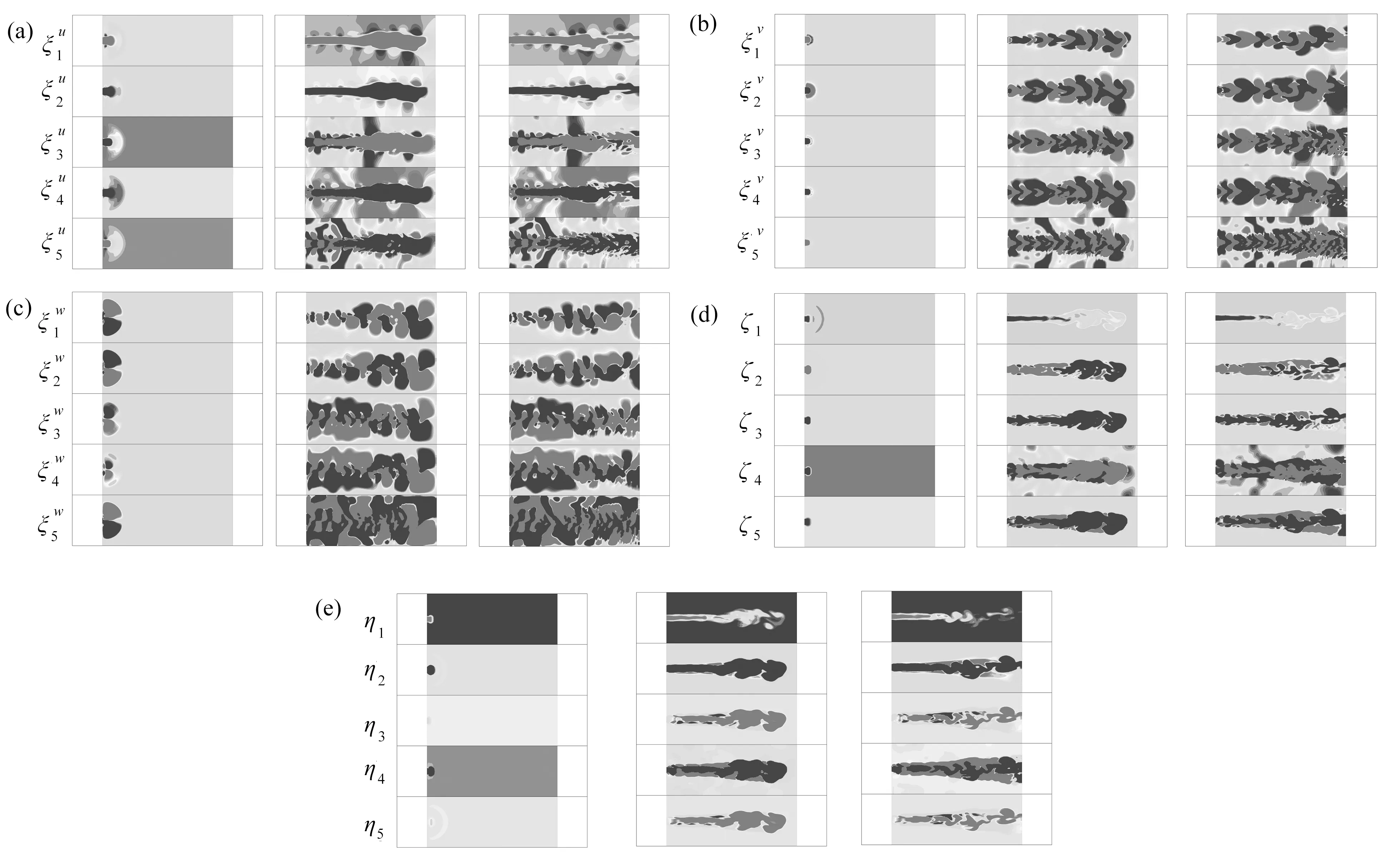
Fig.18 Time evolution of spatiotemporal-coupling optimal velocity basis ξ,density basis ζ and temperature basis η:from left to right,t=100 s,3 000 s,6 000 s
6 Conclusions and the Future Work
6.1 Conclusions
From the above results,one can draw the following conclusions.
First,the concept of traditional spectrum expansion based on the separation of variables and known spatial basis functions is extended to the spatiotemporal-coupling spectrum expansion with the SCOBs satisfying various complex boundary conditions and physical constraints.
Second,the numerical experiment(fig.4)shows that all low-dimensional dynamical system models based on spatial bases are not predictable.
Third,the accurate quantitative comparison between solutions of the SCOLDDS and the CFD for compressible Navier-Stokes equations shows that,the whole field error is typically below 10-2%,and the average error at each cell point is below 10-8%,thus ensuring that the approximate solution of the SCOLDDS is in the attraction domain of the numerical solution of the CFD(and the infinite-dimensional Navier-Stokes equations).Then,the accurate dynamical system characteristics of the Navier-Stokes equations can be obtained through analysis of the characteristics of SCOLDDS.
Fourth,the solution of the SCOLDDS for compressible Navier-Stokes equations can be used to approximate the numerical solution of LES equations,which shows through analysis of the characteristics of the SCOLDDS for the Navier-Stokes equations,the accurate turbulent dynamical system characteristics of the LES equation can be obtained.
Finally,using SCOBs is the key to constructing the SCOLDDS.It can obtain the qualitative analysis results of the dynamical system and be quantitatively compared to real flow with very low-dimensional spatiotemporalcoupling intrinsic bases,to ensure the characteristics of SCOLDDS are the dynamic characteristics of the real flow(such as turbulence).
6.2 The Future Work
The traditional PDE dynamical system models are based on spatial bases,and the objects of dynamical system analysis are limited to the time evolution characteristics of the coefficients of spatial bases,such as bifurcation and chaos.In this study,the modelling theory of SCOLDDS is proposed,and the SCOLDDS model,which is quantitatively comparable to the solution of the infinite-dimensional dynamical system,is obtained,which provides a new research idea and possibility for understanding the characteristics of SCOLDDS for complex flow including compressible turbulence.Therefore,it is necessary to develop a set of corresponding SCOLDDS analysis methods to study the evolution rules and characteristics of complex spatiotemporal-coupling dynamics of real compressible turbulence.
This paper focuses on the modelling theory for OLDDS with spatiotemporal-coupling for compressible flow.The results of the modelling theory of SCOLDDS for incompressible flow will be published elsewhere.
The method of optimal low-dimensional dynamical systems based on spatiotemporal bases is successfully used to the develop a new LES method for compressible turbulent flows,which will published elsewhere.
AcknowledgmentsThe 2nd author extends his appreciation to his former student Mr.WANG Jincheng for his help in this study.
Appendix A The Conjugate Gradient Numerical Optimization Algorithm