HITTING PROBABILITIES AND INTERSECTIONS OF TIME-SPACE ANISOTROPIC RANDOM FIELD

Jun WANG (王军)

School of Statistics and Mathematics，Zhejiang Gongshang University，Hangzhou 310018,China School of Mathematics and Finance，Chuzhou University，Chuzhou 239000,China E-mail : wjun2009@163.com

Zhenlong CHEN(陈振龙)*

School of Statistics and Mathematics,Zhejiang Gongshang University，Hangzhou 310018,China E-mail : zlchenwv@163.com

For Brownian motion, some sufficient and necessary conditions for intersections of the sample paths of stochastic processes were established by Evans [5], Tongring [6], Fitzsimmons and Salisbury [7] and Peres[8]. The hitting probabilities of the random string processes driven by time-space white noise were studied by Chen[9]. Dalang et al. [10]considered intersections of sample paths for Brownian sheets,and Chen and Xiao[11]and Chen et al. [12]for a large class of anisotropic Gaussian random fields. In these papers, the special dependence structures of stochastic processes such as conditional variance and strong local non-determinism play crucial roles.

Recently, various conditions on the density of random vectors were identified naturally in studying the hitting probabilities for a system of stochastic partial differential equations.These conditions are used to study the stochastic heat equations driven by space-time white noise. Dalang et al. [13-15] considered the solutions of the linear stochastic heat equations and the nonlinear stochastic heat equations. Dalang and Pu [16] considered and obtained the optimal lower bounds on hitting probabilities for a system of non-linear stochastic fractional heat equations,and Dalang and Sanz-Sol´e[17]considered the solution of a linear wave equation in all spatial dimensions. Chen[18]studied intersections of the sample paths of two independent random fields under certain general conditions, and he also obtained Hausdorffdimension of the set of intersection times. Ouyang et al. [19] considered a Hausdorffdimension and packing dimension results for the set of intersection times of two independent solutions of stochastic differential equations driven by independent fractional Brownian motions.

Several classes of anisotropic random fields have arisen naturally in the study of random fields and stochastic partial differential equations, as well as in many areas to which they can be applied, including image processing, hydrology, geosatistics and spacial statistics.

Anisotropic random fields are widely studied. It is well known that the fractional Brownian sheets introduced in Kamont[20]is the typical example of a time variable anisotropic Gaussian random field. The characteristics of the polar functions for fraction Brownian sheets were studied by Chen [21]. Another example includes the solution of the stochastic heat equations driven by space-time white noise(see, for example, Chen and Xiao[11], Mueller and Tribe [22],Xiao [23], Wu and Xiao [24]). Examples of space variable anisotropic Gaussian random fields can been found in Adler[25],Xiao[26,27],Didier and Pipiras[28],and Mason and Xiao[29]. Li and Xiao[30]and Ni and Chen[31]constructed and studied a large class of time-space variable anisotropic random fields. When Ni and Chen [32] studied the HausdorffMeasure of the range of anisotropic Gaussian random fields under certain mild conditions, the authors also provided a method for constructing time-space anisotropic random fields. Xiao [33] gave a review of recent progress on anisotropic random fields.

Based on the aforementioned works, in this paper, we study the hitting probabilities and intersections of two independent time-space anisotropic random fields with the general conditions of joint density functions, marginal density functions, and an expectation of moments defined on bounded interval.

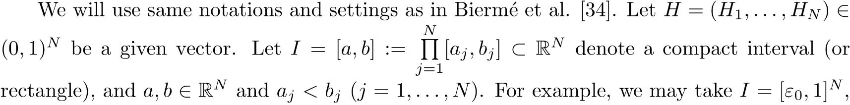
where ε0∈(0,1) is a fixed constant. Let α=(α1,...,αd)∈(0,1]dbe a fixed vector. Without loss of generality, we assume that 0 ＜α1≤α2≤... ≤αd≤1. Note that this assumption is not essential. α will be used to define a space metric on Rd.

Let X = {X(t),t ∈RN} be a random field with continuous sample paths defined on a probability space (Ω,F,P) by

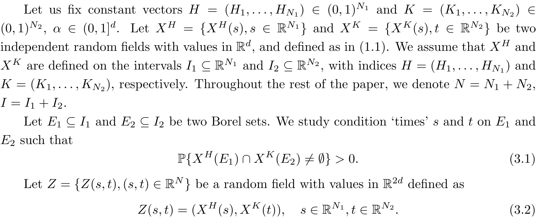
Let XH= {XH(s),s ∈RN1} and XK= {XK(t),t ∈RN2} be two independent random fields taking values in Rdwith indices H =(H1,...,HN1)∈(0,1)N1and K =(K1,...,KN2)∈(0,1)N2, respectively. We say that the two random fields XHand XKintersect if there exist s ∈RN1and t ∈RN2such that XH(s) = XK(t). In this paper, we address the following problems that are concerned with existence of intersections:

(i) When do XHand XKintersect with positive probability?

(ii) Let E1⊆RN1and E2⊆RN2be arbitrary Borel sets. When do XHand XKintersect if we restrict the ‘time’ s ∈E1and t ∈E2? That is, when is

The rest of the paper is organised as follows: in Section 2 we study the hitting probabilities of random field X. In Section 3 we study Questions (i)-(iii). We give an example of an anisotropic non-Gaussian random field in Section 4. Throughout this paper we will use c to denote an unspecified positive and finite constant which may not be same in each occurrence.More specific constants are numbered as c1,c2,... .

2 Hitting Probabilities

In this section, we consider the hitting probabilities of random fields defined as(1.1)under some general conditions. We first briefly recall the Hausdorffdimension and the Bessel-Riesz type capacity, then give some Lemmas, and finally give the main result (Theorem 2.5). We note that Chen and Xiao[11]considered the problem of hitting probabilities of time anisotropic Gaussian random fields under moment and conditional variance, and their results refined the corresponding results in Bierm´e, Lacaux and Xiao [34] and Xiao [23]. For systems of linear stochastic fractional heat equations in spatial dimension 1 driven by space-time white noise,the question of hitting points was studied by Wu[35]. Later,Chen and Zhou[36]considered the problem of hitting probabilities of inverse images of a class of time anisotropic random fields.Ni and Chen[31]and Chen et al. [12]studied the hitting probabilities of time-space anisotropic Gaussian random fields.

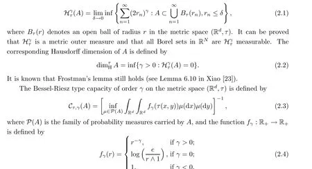
For any constant γ >0 and set A ⊆Rd, define the γ-dimensional Hausdorffmeasure with the metric τ of A as

In addition, we define the metricon RN×Rdas

Next we give some lemmas. Lemma 2.1 comes from Lemma 2.1 of Ni and Chen [31].

Lemma 2.1 Suppose that d is a positive integer, and 1 ≤β1≤β2≤...βd＜∞, ai≥0 for all i=1,...,d. Then,

(i) if ai≤1 for all i ∈{1,2,...,d}, there exists a positive constant c6such that

(ii) if there exists i ∈{1,2,...,d}such that ai≥1, there exists a positive constant c7such that

The following lemma is a result about small ball hitting probability of X and will be used in the proofs of Theorem 2.5 and Theorems 3.2 and 3.4:

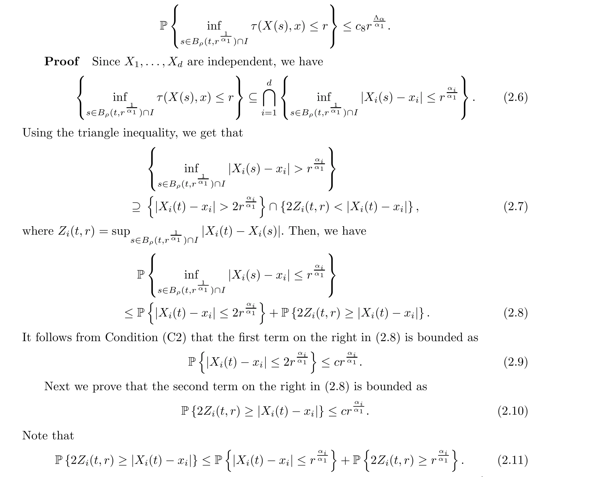
Lemma 2.2 Let X be an (N,d)-random field defined by (1.1). If X satisfies Conditions(C2) and (C3), then for any constants M > 0, 0 ＜r0＜1, there exists a positive constant c8depending on H,N,α,d and M only, such that, for all x ∈[-M,M]d, r ∈(0,r0) and t ∈I,

Now we divide the proof of (2.16) into three cases.

Case 1. If ρ(s,t)α1≤τ(x,y) and if, for any 1 ≤i ≤d, we have that |xi-yi|2≤ρ(s,t),then by (2.18) and (i) in Lemma 2.1, we have

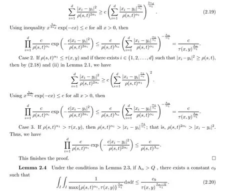
Proof By the proofs (2.37)-(2.39) in Ni and Chen [31], we get the conclusion. □

The next theorem is the main result in this section. We consider the hitting probabilities of time-space random field X under some general Conditions (C1)-(C3).

Theorem 2.5 Let X be an (N,d)-random field defined by (1.1) satisfying Conditions(C1)-(C3). If Λα>Q, E ⊆I and F ⊆Rdare Borel sets, then

Combining Condition (C1), Lemma 2.3, Lemma 2.4 and (2.4), we have

where (F)(ε)denotes the closed ε-enlargement of F, and the path of X is continuous, letting ε ↓0, we get the lower bound in (2.21). This finishes the proof. □

Remark 2.6 According to Theorem 2.5, it would be of interest to study the fractal dimensions of the level set of X. With our conclusions in hand, we will study in a future paper about fractal dimensions of the level sets of X under the density function conditions with different space metrics.

3 Intersections

In this section, we use the estimation of the small ball probability of anisotropic random fields obtained in Section 2 under some general conditions to study Questions(i)-(iii). Note that Chen and Xiao[11]and Chen et al. [12]considered the problems(i)-(iii)of time anisotropic and time-space anisotropic Gaussian random fields,respectively. Chen[37]studied the existence and fractal dimension of intersection of nondegenerate diffusion processes. Chen[18] considered the time anisotropic random fields. Ouyang et al. [19]studied the intersections of rough differential systems driven by fractional Brownian motions.

3.1 Questions (i) and (ii)

Then, Question (3.1) is equal to saying that for any given interval G ⊂Rd,

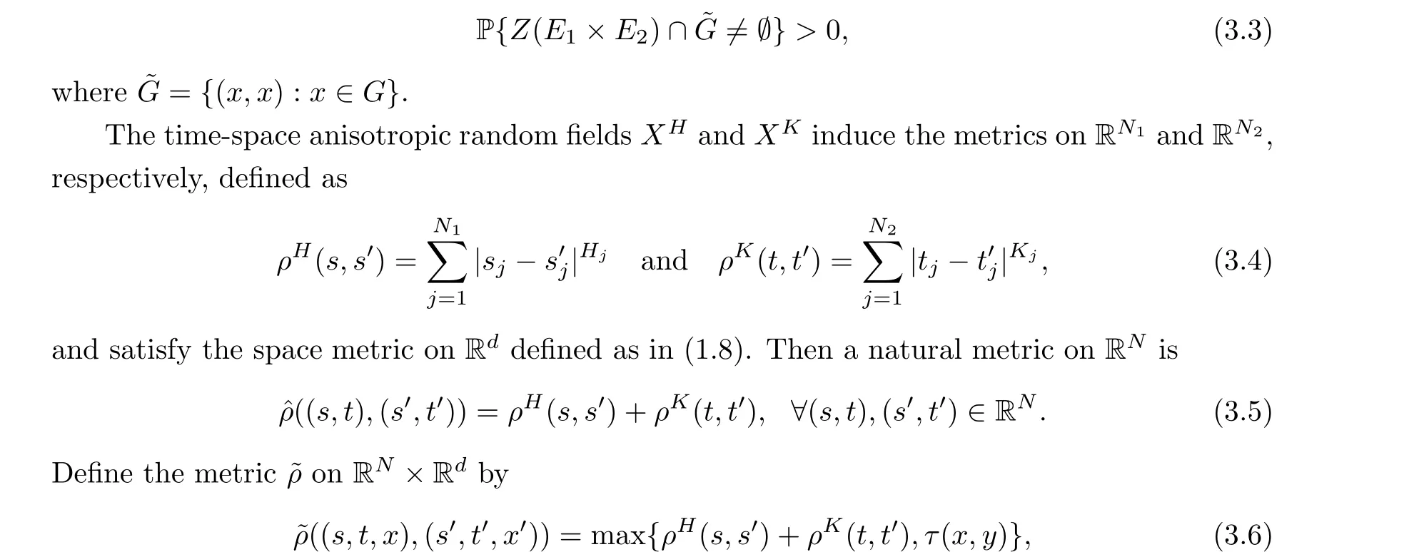
where (s,t),(s＇,t＇)∈RNand x,x＇∈Rd.

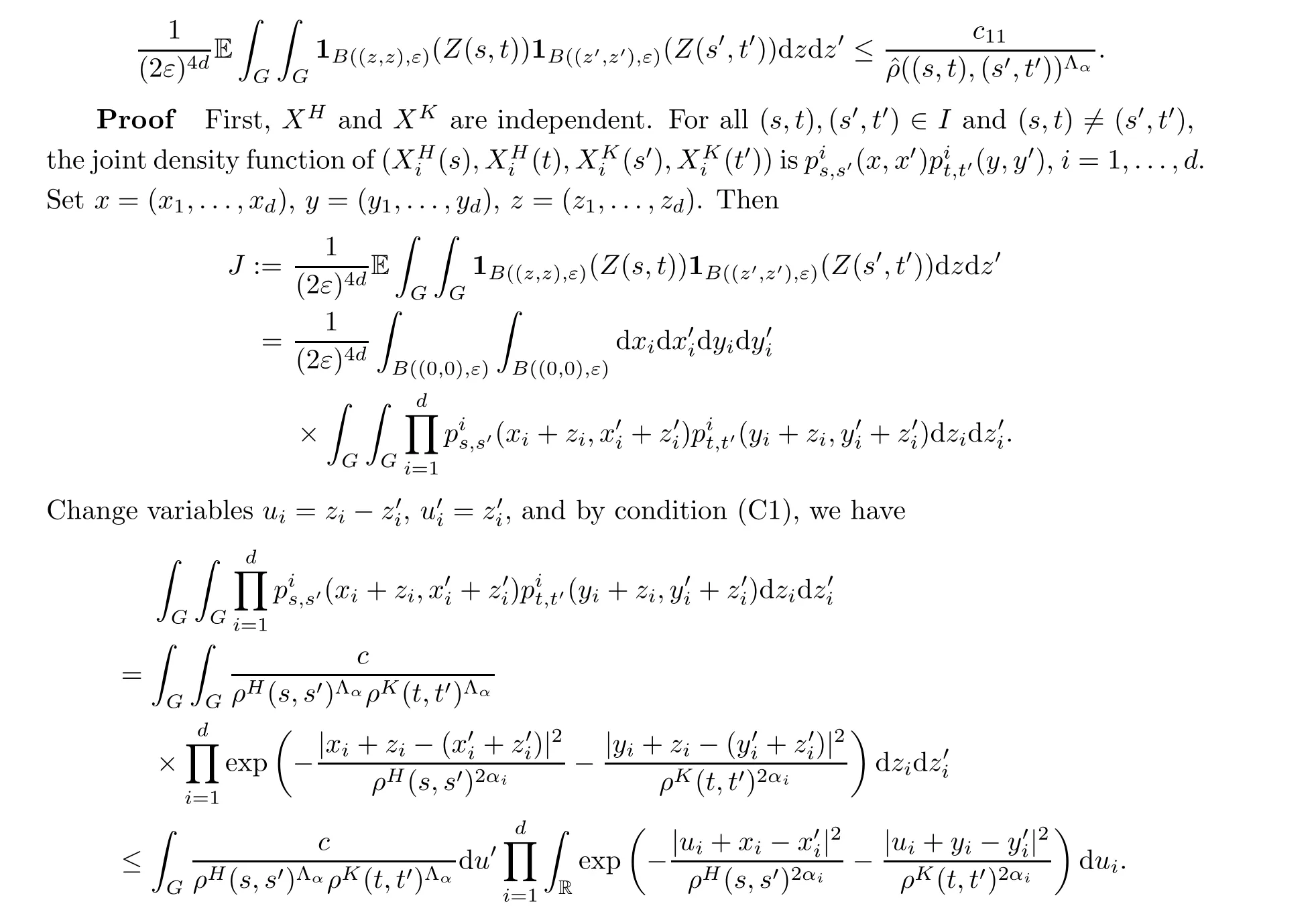
In order to prove the lower bounds in Theorems 3.2 and 3.4, we need following auxiliary lemma:

Lemma 3.1 Let XHand XKbe two independent random fields defined as above and satisfying Condition (C1). Letting any G ⊂Rd, there exists a constant c11such that for all ε ∈(0,1), (s,t),(s＇,t＇)∈I,

3.2 Question (iii)

Now we answer Question (iii). We continue to use the same notations and assumptions as in the first paragraph in Section 3.1.

Let E1⊆I1,E2⊆I2be compact sets,both with positive Lebesgue measure,and let F ⊆Rdbe a Borel set. Now we ask: when does F contain intersection points of {XH(s),s ∈E1} and XK(t),t ∈E2}? That is, when is

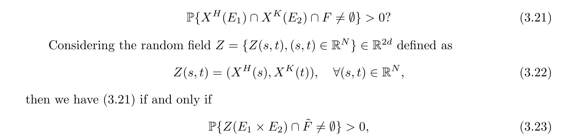
where ˜F ={(x,x):x ∈F}⊆R2d.

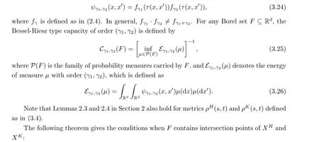
Note that, if H /=K, the component processes XHand XKin Z are not independent and identically distributed. For any constants γ1and γ2, define kernel ψγ1,γ2:Rd→R+as

Theorem 3.4 Let XH= {XH(s),s ∈RN1} and XK= {XH(t),t ∈RN2} be two independent random fields and let both have values in Rdsatisfying Conditions (C1)-(C3). Then,for any compact sets E1⊆I1and E2⊆I2with positive Lebesgue measure and any Borel set F ⊆Rd,

In a fashion similar to the argument of (3.16), we will prove the following two inequalities:

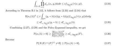
Taking a similar argument as to that of (2.36)and(2.37),and combining(3.34), (3.36)and the Paley-Zygmund inequality, we prove the lower bound in (3.28). This finishes the proof. □

4 Example

As an example of anisotropic non-Gaussian random fields,we show a random field satisfying Conditions (C1)-(C3) with density functions defined on a bounded interval.

Let 1 ＜γ ≤2. Consider a system of non-linear stochastic fractional heat equations with vanishing initial conditions on the whole space R; that is, for i=1,...,d, t ∈[0,T], x ∈R,

where u := (u1,...,ud), with initial conditions u(0,x) = 0 for all x ∈R. Here ˙W :=( ˙W1,..., ˙Wd) is a vector of d independent space-time white noises on [0,T]×R defined on a probability space (Ω,F,P). For all 1 ≤i,j ≤d, the functions bi,σi,j: Rd→R are globally Lipschitz continuous. The fractional differential operator Dγ(1 ＜γ ≤2) is given by

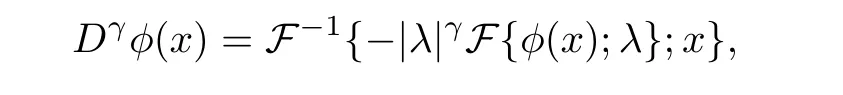
where F denotes the Fourier transform. The operator Dγcoincides with the fractional power γ/2 of the Laplacian. When γ = 2, it is the Laplacian itself. For 1 ＜γ ＜2, it can also be represented by

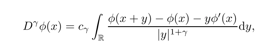
with a certain positive constant cγdepending only on γ. We can refer to Dalang and Pu [16]and Kwa´snicki [38] for addition equivalent definitions of Dγ.

A mild solution of (4.1)is a jointly measurable Rdvalued process u={u(t,x),t ≥0,x ∈R}such that, for i=1,...,d,

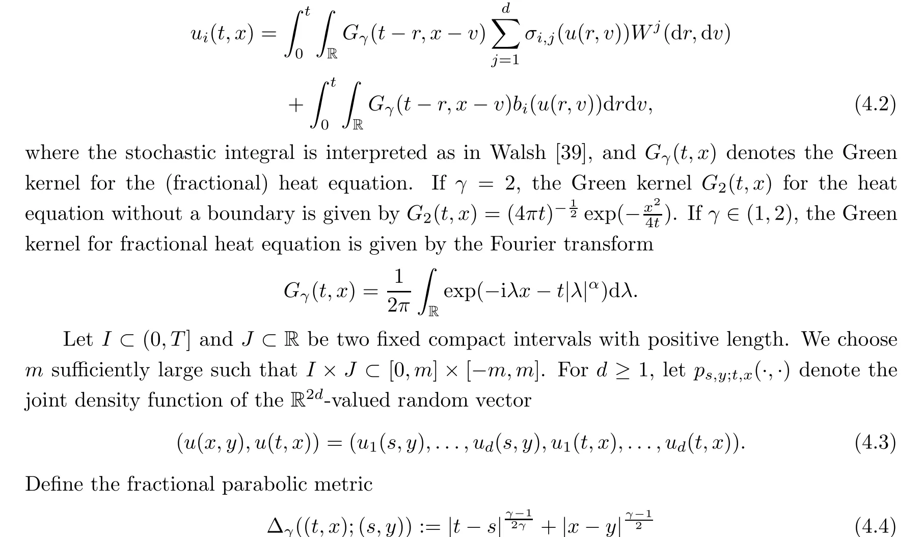
for s,t ∈[0,T] and x,y ∈R.

Dalang and Pu [16] studied the non-linear systems of stochastic fractional heat equations(4.1). They established a sharp Gaussian-type upper bound on the two-point probability density function of (u(s,y),u(t,x)) with metric (4.4) (see Theorem 1.1 in Dalang and Pu [16]). Then they deduced optimal lower bounds on the hitting probabilities of process {u(t,x) : (t,x) ∈[0,∞)×R} in the non-Gaussian case, which improves the results in Dalang et al. [14] for systems of classical stochastic heat equations.

With these preparations, we consider the random field u = {u(t,x),t×x ∈[0,T]×[0,1]}with values in Rddefined as

where the coordinate processes u1,...,udare independent. For i = 1,...,d, uiis the solution of equation (4.1).

Theorem 4.1 shows that the random field u in (4.5) satisfies Conditions (C1)-(C3) with H1= 1/4, H2= 1/2 and α1= ... = αd= 1. Hence our results are applicable to anisotropic non-Gaussian solutions of non-linear systems of stochastic fractional heat equations.