
Modified Differential Transform Method for Solving Black-Scholes Pricing Model of European Option Valuation Paying Continuous Dividends
2023-02-15 06:39AHMADManzoorMISHRARajshreeandJAINRenu
AHMAD Manzoor*,MISHRA Rajshree and JAIN Renu
1 School of Mathematics and Allied Sciences,Jiwaji University,Gwalior-474011,India.
2 Govt.Model Science College,Gwalior-474011,India.
Abstract. Option pricing is a major problem in quantitative finance.The Black-Scholes model proves to be an effective model for the pricing of options.In this paper a computational method known as the modified differential transform method has been employed to obtain the series solution of Black-Scholes equation with boundary conditions for European call and put options paying continuous dividends.The proposed method does not need discretization to find out the solution and thus the computational work is reduced considerably.The results are plotted graphically to establish the accuracy and efficacy of the proposed method.
Key Words: European option pricing; Black-Scholes equation; call option; put option; modified differential transform method.
1 Introduction
The financial agreements made between buyers and sellers in the financial markets is known as option pricing.It accounts for numerous purposes for example to hedge assets and portfolios to minimize or to control the risk due to variability in stock prices.There are varied mathematical models available for pricing different types of options.The problem for pricing options was mathematically modeled first in 1973 by Fisher Black and Myron Scholes[1]on European or American call(right to buy)and put(right to sell)options.European options are traded only on a specified future date before expiry while American options are exercised or traded at any time up to the expiry.
The Black-Scholes model is mainly based on the concept of constructing a risk-less portfolio taking into account the bonds,option and the underlying stock.Moreover,it also takes into consideration the concept of hedging and eliminating risk of option pricing for purchasing and selling of underlying assets.The Black-Scholes option pricing model is based on the assumption that the underlying asset does not pay any dividends during the life time of the option.Merton [2] extended the Black-Scholes option pricing model to underlying assets that pay a continuous dividend yield during the life time of the option and derived the modified Black-Scholes equation and the modified Black-Scholes formulae for both European call and put options.The Black-Scholes model for the valuation of European options paying continuous dividend yield is given by the partial differential equation:
whereV(S,t)is the option price or option premium at asset priceSand at timet,S(t)is the asset price at timet,σrepresents the volatility,ris the risk free interest rate andDis the dividend yield.
Let us denote the value of European call and put options byVc(S,t) andVp(S,t) respectively.Then the pay off functions for European call and put options are given by:
whereKdenotes the strike price.It is well known that Eq.(1.1)has a closed form solution depending on the fundamental solution of heat equation.Hence,it becomes necessary to transform the Back-Scholes equation to a heat equation after certain change of variables.After finding the closed form solution of the heat equation,it can be transformed back to find the solution of the Black-Scholes partial differential equation[3].
Since the classical Black-Scholes equation was established under some strict assumptions,a wide class of analytical and numerical methods has been proposed from time to time to weaken these assumptions such as Laplace method [4,5],Fourier transform method[6],iteration method[7],homotopy perturbation method[8-10],variational iteration method[11],new iterative method[12],homotopy analysis method[13],Adomian decomposition method[14]and differential transform method[15].
The main aim of this paper is to extend the application of modified differential transform method to obtain the approximate analytical solution of Black-Scholes European call and put options paying continuous dividends.The differential transform method was first applied by Zhou in 1986 in the field of engineering to solve linear and nonlinear equations in electrical circuit analysis[16].Several authors have further modified the differential transform method and applied it to certain differential equations both linear and non-linear in nature.The modified differential transform method is one such method that can be applied to solve differential equations without linearization or perturbation[17].
In this paper the Black-Scholes model based on European call and put options paying continuous dividends has been studied.The solution is carried out by a reduced differential transform method known as the modified differential transform method.The rest part of this paper is organized as follows: in Section 2,the basic definitions,fundamental operations and properties of differential transform method and modified differential transform method are given; in Section 3,the Black-Scholes equation for pricing European call and put options paying continuous dividends is given;in Section 4,the Black-Scholes equation for European call and put options have been solved through modified differential transform method.The computational results have been obtained through MATLAB and are discussed in Section 5.Finally,we have presented the conclusion in Section 6.
2 Differential transform method and modified differential transform method
2.1 Differential transform method
The basic definitions and fundamental operations of two-dimensional differential transform method are defined as follows[18]:
Ifv(x,τ)is analytic and continuously differentiable with respect to timeτand spacexin the domain of interest,then,the differential transform ofv(x,τ)is given as:
and its inverse differential transform is defined as
Using Eq.(2.1)in(2.2),we get:
It is shown that the differential transform method is easier in terms of application when solving both linear and non-linear differential equations.The solution obtained through this method is based on Taylor series.Even though this method proves useful over other semi-analytical methods,some level of difficulty is still met when dealing mainly with the nonlinear differential equations and differential equations with variablecoefficients which provides a room to modify the differential transform method[19,20].
The modified differential transform method is a modification of differential transform method used to solve both linear and non-linear differential equations.The basic definition and fundamentals of modified differential transform method are given as follows:
2.2 Modified differential transform method
If the functionv(x,τ) is analytic and continuously differentiable with respect to timeτand spacexin the domain of interest then[17]:
Herev(x,τ)is the original function andV(x,m)stand for the transformed function.The differential inverse transform ofV(x,m)is given as:
Combining Eqs.(2.4)and(2.5)we get:
It can be deduced that modified differential transform method is derived from power series expansion.The fundamental properties of modified differential transform method are given in Table 1.
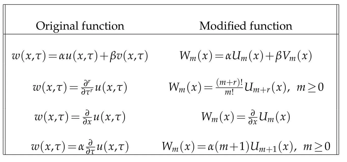
Table 1: Modified Differential Transform Method
3 The Black-Scholes equation for pricing European call and put options paying continuous dividends
The fair price of European options on a single underlying asset paying continuous dividends yield is given by Black-Scholes partial differential equation[2].
whereV(S,t)is the option price or option premium at asset priceSand at timet,S(t)is the asset price at timet,σrepresents the volatility,ris the risk free interest rate andDis the dividend yield.The boundary options for call options are:
and the boundary conditions for put options are:
The final condition for call options is
And the final condition for put options is
The first thing to do is to get rid of the awkwardSandS2terms multiplyingandin Eq.(3.1).
At the same time we take the opportunity of making Eq.(3.1) dimensionless as defined in the technical point below,and we turn it into a forward equation.We set:
Applying the above transformations in Eqs.(3.1) to (3.5),the Black-Scholes equation reduces to:
4 Solution of Black-Scholes equation through modified differential transform method
Consider the Black-Scholes equation for European call options paying continuous dividend yield
subject to initial condition:
To solve Eq.(4.1)in view of Table 1,we obtain the following recurrence formula:
In view of modified differential transform method,Eq.(4.2)can be written as:
Taking the derivative of Eq.(4.5),we get:
Form=0,1,2,3,...,we have:
Therefore,
Therefore,
Therefore,
In this way we get:
Hence,the solution through modified differential transform method is given in a series form as:

Figure 1: (a) MDTM solution plot for k1=2 and k2=2; (b) MDTM solution plot for k1=10 and k2=5.
Thus the exact solution of Eq.(4.1)is given as:
Particular case
For the particular case,k1=k2=kwe get:
which is an exact solution of classical Black-Scholes equation and is similar to the results obtained in[17]and[21].
5 Computational results
In this section,the series solution of above B-S model is computed numerically.
In Fig.1(a),the surface plot of European call option computed through MDTM is drawn for parametersk1=2,k2=2 over a range of 0≤x≤4.The time parameterτranges from 0≤τ≤6.The option price increases with increasingx.With increasingxfrom 0-1,the option price approaches to zero.After that the value ofvincreases exponentially.The results show that with higher value ofxand with more time to expiry,vhas a higher value.The value ofvdecreases with less time to maturity.Fig.1(b)represents the surface plot for parametersk1=10 andk2=5 over a range of 0≤x ≤4 and 0≤τ ≤6.The option price reaches to zero with increasingxfrom 0-1.After that the value of option shows a significant increase asxincreases from 1-4.The results show the value ofvincreasing with increasingxand with more time to maturity.
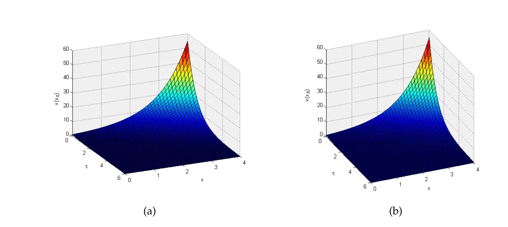
Figure 2: (a) MDTM solution plot for k1=5 and k2=4; (b) MDTM solution plot for k1=6 and k2=5.
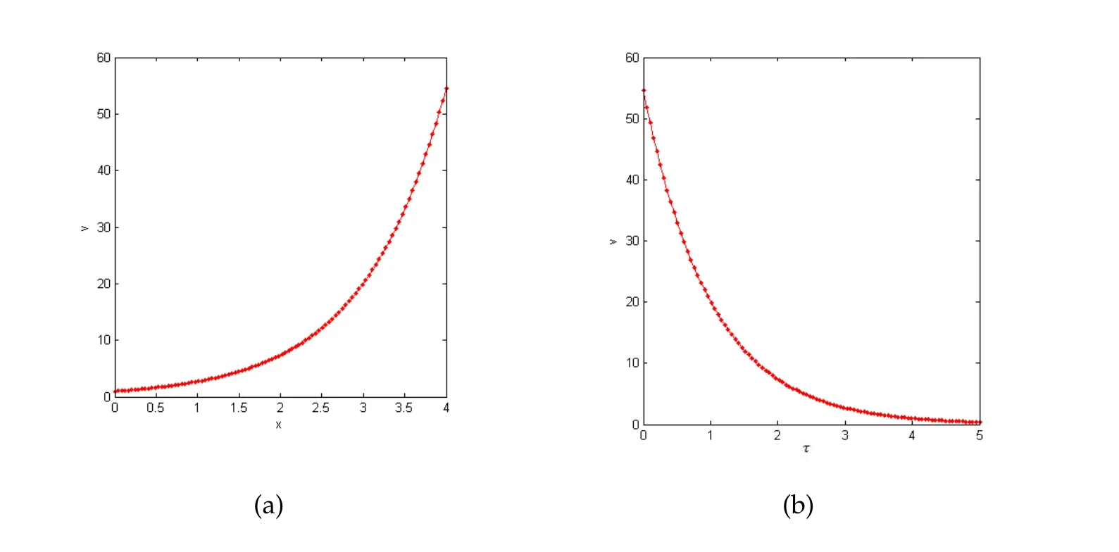
Figure 3: (a) MDTM solution plot for k1=2 and k2=2, τ=4 and (b) MDTM solution plot for k1=3 and k2=2, x=4.
Fig.2 is computed for different values ofk1andk2.The results follow the same trend as given in Fig.2.
Fig.3(a)shows the plot of European call option.The solutionvis computed forxwith fixedk1=2,k2=2 andτ=4.The results show that the value ofvincreases significantly asx >2 and attains the maximum value atx=4.The numerical analysis show that the value ofxhas a significant impact on the value of the option price.Fig.3(b)shows the plot of European call option with parametersk1=3,k2=4.The valuevis computed for fixedx=5 withτranging from 0≤τ ≤5.It is shown that as the time period decreases,the value of option also decreases and approaches to zero as the time period reaches to expiry.

Figure 4: (a) MDTM solution plot for k1=5 and k2=4, τ=4 and (b) MDTM solution plot for k1=10 and k2=5, x=4.

Figure 5: (a) Comparison of MDTM solution with PDTM solution given in [17] for k1=0.8, k2=0.6, k=0.6,τ=2 and (b) Comparison of MDTM solution with ADM solution given in [21]k1=1, k2=2, k=1, τ=2.
Fig.4(a) shows the MDTM solution plot fork1=5,k2=4 andτ=4.The value ofxranges from 0-4.It is clearly shown that for greater value ofk1thank2,the value ofvdecreases and increases exponentially ask2>k1.In Fig.4(b),the MDTM solution is computed for fixedx.The results again clearly indicate thatvdecreases with decreasingτand approach to zero as time approaches to expiry.
Fig.5(a) shows the comparison of solutions obtained through MDTM and PDTM given in[17]and Fig.5(b)shows the comparison of solutions obtained through MDTM and ADM given in[21].
In Table 2,the analysis of the MDTM solution is presented and compared to the solution obtained through PDTM for non dividend paying options given in[17].The comparison is in terms of computing the exact solutions numerically.
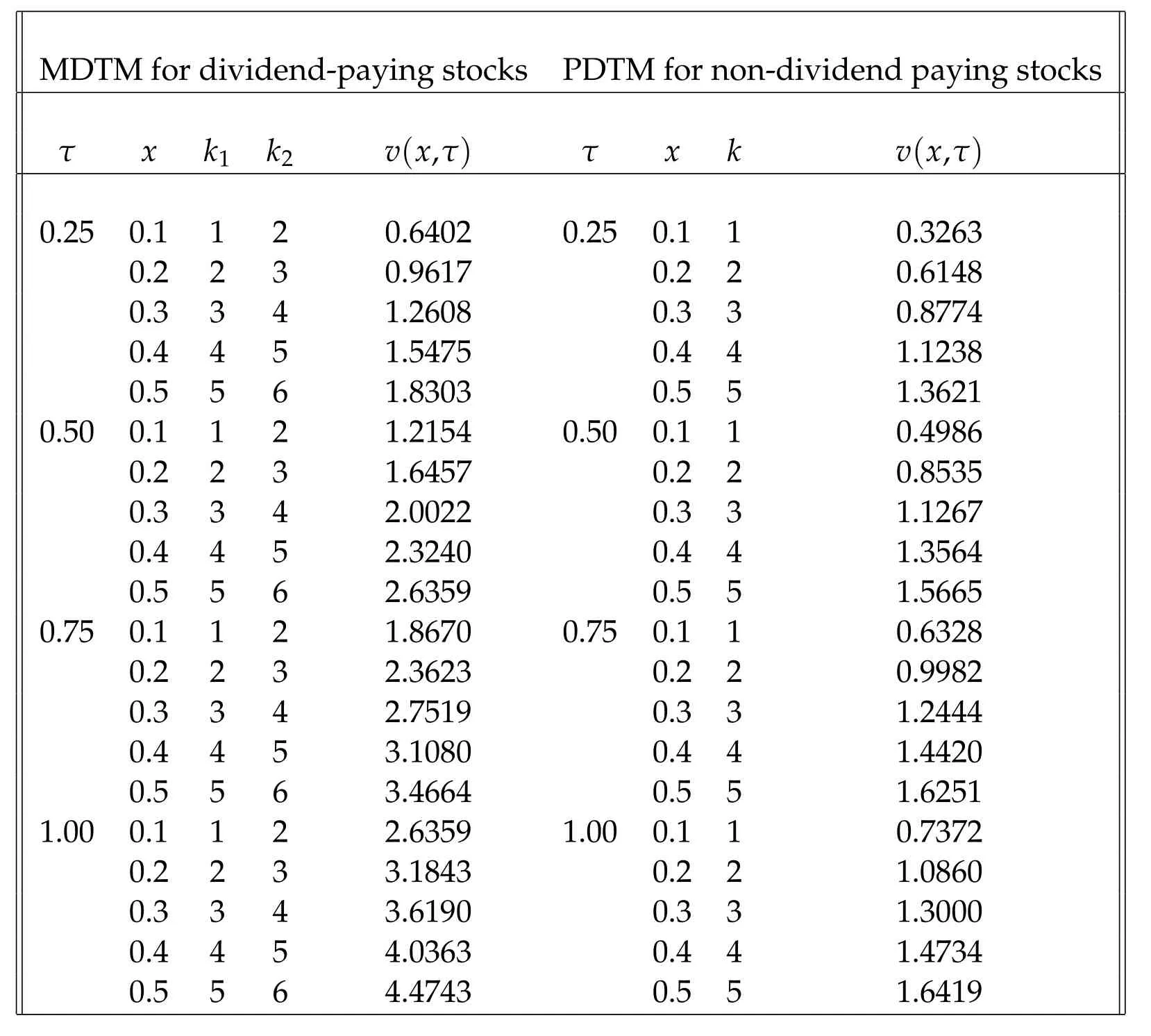
Table 2: Comparison of numerical results obtained through MDTM on a dividend paying asset with PDTM solution on a non-dividend paying asset given in [17].
6 Conclusions
In this paper,we have successfully applied the modified differential transform method(MDTM)for the first time to solve Black-Scholes pricing model of European call and put options paying continuous dividends.The obtained results are computed through MATLAB and are compared to the results obtained through projected differential transform method(PDTM)and Adomian decomposition method(ADM)for non-dividend paying options [17,21].It is well found that this method is very simple in application and at the same time gives better results as compared to other methods.The results are obtained from a recursive relation and arbitrary numbers can be obtained in terms of series expansion of solution.This method can be applied to linear and non-linear differential equations without discretization or linearization.It can also be observed from Table 2,as the value ofx,τ,k1,k2increases,the value ofvalso increases and the call option can be exercised.Moreover,this method can be easily applied to generate novel applications in the field of applied science and engineering.The same algorithm can be applied on European put options.The results are presented graphically to demonstrate the efficiency and effectiveness of the proposed method.
 Journal of Partial Differential Equations2023年4期
- Journal of Partial Differential Equations的其它文章
- A Diffusive Predator-Prey Model with Spatially Heterogeneous Carrying Capacity