The performance of a dissipative electrooptomechanical system using the Caldirola-Kanai Hamiltonian approach

M M Atabaki,M K Tavassoly,A Behjat,∗,M Hassani Nadiki and K Javidan

1 Optics and Laser Group,Faculty of Physics,Yazd University,Yazd,Iran

2 Department of Physics,School of Sciences,Ferdowsi University of Mashhad,Mashhad 91775-1436,Iran

Abstract

By combining all optical,electronic,and mechanical capabilities,electro-optomechanical systems,along with the use of mechanical displacement,the conversion of low-frequency electrical signals into much higher-frequency optical signals is possible.This process provides several capabilities that have very important applications in various fields,including classical,as well as quantum communications.In this regard,the inevitable effect of dissipation on the performance indicators of such systems is one of the important issues affecting its efficiency.One approach for investigating the effect of dissipation is based on a time-dependent Hamiltonian has been known as the Caldirola-Kanai (CK) Hamiltonian,wherein the exponentially increasing mass,i.e.m (t)=m0 eγtenters the mechanical oscillator system.Utilizing this approach shows that,the performance of the system under the influence of dissipation with CK Hamiltonian formalism,in which the dissipation terms are embedded in the Hamiltonian,are more logical,analytical,and reliable than considering the effect of dissipation with the phenomenological method(including the dissipation effects in the equations of motion by hand),which has been recently used in Bagci et al.(Nature,507,81,2014).In our method,it is also possible to monitor the performance of the system via the adjustment of dissipation components,i.e.,resistance R and reactance L (and CK damping parameterγ) in the electrical(mechanical membrane) part of the system.

Keywords: dissipative system,electro-optomechanical system,Caldirola-Kanai Hamiltonian

1.Introduction

The conversion of radio waves to optical waves with higher frequencies enables one to transmit the radio waves through optical fiber with very low losses.This conversion provides access to a set of existing quantum optics capabilities[1].On the other hand,the role of mechanical displacement has attracted a lot of attention in many fields [2].The electrical drive of moving parts in optical cavities or optical waveguides can be used to adjust the phase or frequency of the corresponding optical field to create an effective electrooptical interaction.This interactive interaction can be performed in two ways.The force exerted by light,i.e.,the radiation pressure created by a light beam that is reflected by a mirror may cause mechanical displacement; conversely,the displacement may induce voltage and current in a piezoelectric material or a capacitive sensor [3].The combination of optical,electronic,and mechanical capabilities,along with the use of mechanical displacement characteristics,provides new applications from the electrical tuning of optical and mechanical devices to the bidirectional conversion of microwave and optical quantum signals.By combining all the abovementioned capabilities,electro-optomechanical systems enable one to convert low-frequency electrical signals into much higher frequency optical signals.This conversion process provides very important applications in astronomy,medical imaging,navigation,and classical as well as quantum communication.For instance,it enables modern communication networks to use both the strengths of electrical circuits and optical connections,and thus information networks can be tuned in size and complexity [1,3].

Such systems consist,in general,of two electrical and optomechanical subsystems,wherein by combining electromechanical and optomechanical technologies,a mechanical resonator is simultaneously coupled to both the electrical circuit and the optical cavity.These simultaneous connections lead to the flowing of the radio signal through the mechanical resonator,which appears as light waves [3-5].Several parameters can be taken into consideration to investigate electrooptomechanical systems as performance indicators of the system.In particular,the effect of dissipation on the system performance is one of the important issues that particularly affects its efficiency.Recently,in a pioneering paper,considering an electro-optomechanical system,the effect of dissipation has been taken into account,using a phenomenological approach [5].However,another candidate to investigate the effect of dissipation is to use of the time-dependent Hamiltonian known as the Caldirola [6]-Kanai [7] (CK)Hamiltonian.In fact,briefly,the CK Hamiltonian has been used to describe the dissipative harmonic oscillator system(with exponentially increasing massm(t)=m0eγt).Lewis and Riesenfeld [8,9] using the CK Hamiltonian have introduced an invariant operator in order to treat time-dependent Hamiltonian systems.Shortly after,this approach became a very useful tool in revealing the quantum theory of these systems [10-16].Denisova and Horsthemke investigated the statistical properties of damped quantum particles using the CK method and presented a new method for solving the timedependent Schrödinger equation [10].Um et al showed that the path integral approach yields the exact quantum theory of the CK Hamiltonian without violating the Heisenberg uncertainty principle,based on which the authors presented exact quantum theories for various dissipative harmonic oscillators [11].Choia and Yeon have studied the coherent states of an inverted CK oscillator with time-dependent singular potentials using the constant operator method and the Lie algebra approach [12].Recently,Choi investigated the quantized energy for the CK Hamiltonian systems in coherent states,based on constant operator theory [15].Sanz et al presented a Bohemian analysis of friction dynamics to achieve how a hypothetical and purely quantum viscous medium acts on a wave packet from a hydrodynamic quantum point of view [16].

In this paper,we use the CK Hamiltonian approach in the considered electro-optomechanical system.The results of investigating the performance of the system under the influence of loss with the aforementioned Hamiltonian CK approach show that,in general,the results are logical,analytical,and more reliable than considering the effect of loss with the phenomenological method.For instance,with our method,it is possible to analyze the performance of the system due to the change of real loss components in the system (membrane mass,resistance,and inductor inductance),a task that is not so clearly possible in the phenomenological method.While we compare our obtained results with the outcomes of [5] in general,it is also noticeable that,in the continuation of the paper we extract a relationship for the system efficiency depending on the mechanical and electrical bare susceptibilities(and consequently the main loss components) of the system.Accordingly,we are able to analyze the efficiency of the system,in which the appropriate supply voltage range for efficiency is also specified(10-160 V).In addition,based on our numerical results,in order to have enough efficiency,the value of the electrical circuit resistance of the system should be less than 25 Ω,and by reducing it from this value,the efficiency can be increased.

This paper is organized as follows.In the next section,a general description of the electro-optomechanical system is discussed.Section 3 deals with the CK dissipative electrooptomechanical system.Then,the performance indicators of our dissipative electro-optomechanical system are compared with the case with the phenomenological approach,and finally,conclusions are drawn in the final section.

2.A brief review of electro-optomechanical systems

The electro-optomechanical system generally consists of two electromagnetic oscillators,one in the optical frequency and the other in the microwave frequency,which share a mechanical oscillator.The mechanical oscillator consists of a thin silicon nitride membrane that can vibrate (figure 1).The optical oscillator consists of a Fabry-Perot cavity with a variable capacitor inside it.The conversion of an electromechanical signal into an optical signal is done by the dual role of the capacitor,which is not only an element in the electrical circuit but also plays the role of a movable mirror in the optical cavity (constructing an optomechanical system).As is shown in figure 1,the capacitorC(x),consists of a membrane plate that can oscillate(determined byxmeasured from its equilibrium position),while another plate is fixed.The movable plate of the capacitor (the membrane) receives the optical beam radiation pressure.Therefore,the value of the capacitance,denoted byCin the optomechanical equilibrium state,transforms toC(x) in the electro-optomechanical state.The vibrations of the membrane and the reciprocation of the light wave move in the same direction,and thus,the resonance frequency of the optical cavity is modulated[17,18].This membrane is covered with a thin layer of niobium (which is a superconductor at temperatures below 9 K) that is part of the capacitor in a magnetic circuit and forms a microwave resonator [17-19].

Recently,Bagci et al presented an electro-optomechanical system capable of receiving low-frequency electromagnetic signals and converting them into optical signals(with high frequencies) [5].This system is one of the most sensitive electro-optomechanical systems in detecting,receiving,and converting low-to high-frequency signals.The model is described in figure 1.This system consists of optoelectrical as well as optomechanical subsystems.The vibrating membrane forms the oscillating plate of a variable capacitor coupled to an electrical resonant circuit.By placing the variable capacitor inside an optical cavity and applying a voltage of less than 10 V to the electric circuit,a strong coupling between the voltage fluctuations in the electric resonance circuit and the displacement of the membrane can be induced.At the same time,the membrane displacement is coupled to the light reflected from its surface.The movement of the membrane leads to a phase change in the light passing through it.In fact,the membrane oscillations,which are produced by applying an electrical signal,appear as an optical phase change with which a reasonable quantum sensitivity can be detected.The capacitanceCm(x),depends on the distance between the membrane electrodes,d+x,and its dielectric constant.Considering the adjustment capacitorC0in the electric frequency circuit,the total capacity of the capacitor is equal toC(x)=C0+Cm(x),whereCm(x)=withAis the area of the capacitor electrode,dis the distance between the capacitor plates,andxis the displacement of the membrane.

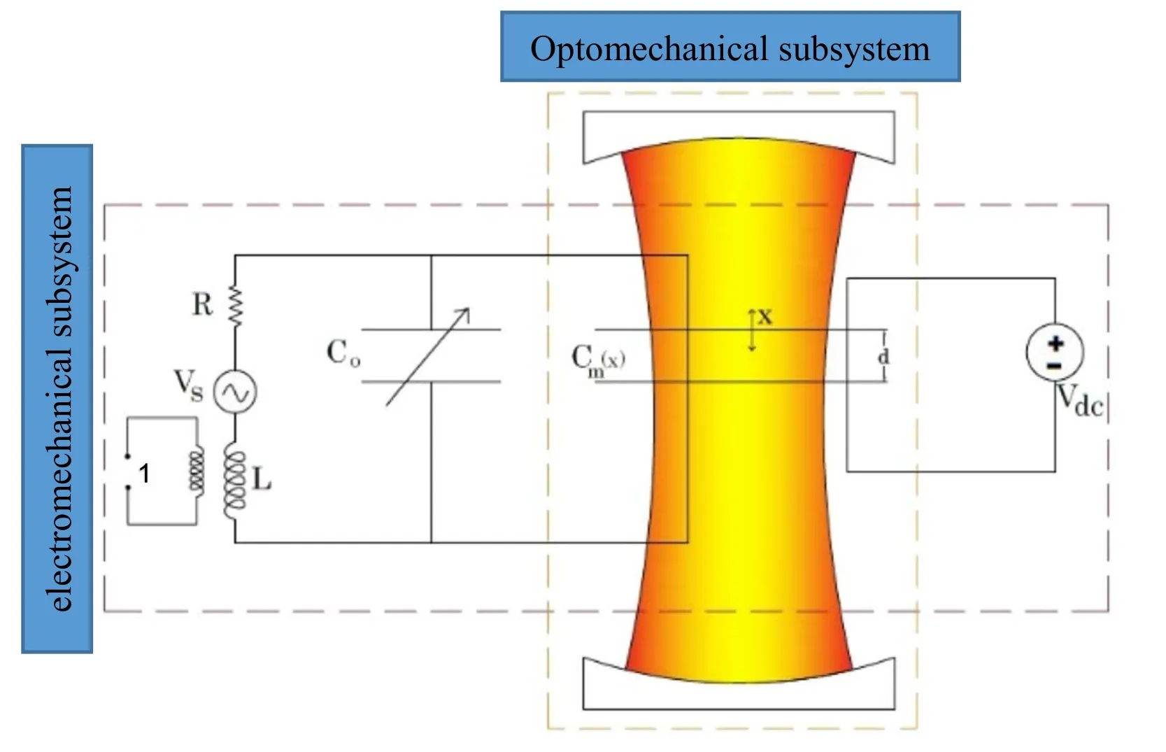
Figure 1.Schematics of the electro-optomechanical system:the movement of light in the cavity is in the same line with the oscillation of the membrane(the upper plate of the capacitorCm).The displacement of the membrane transforms into a phase shift of the laser beam reflected from the membrane.The membrane capacitor is part of the LC circuit,which is tuned with the mechanical resonance frequency by adjusting a capacitorC0.The bias voltage,Vdc,couples the LC circuit to the movement of the membrane.The circuit is driven by a voltage,Vs,which can be injected through the coupling port 1 or taken by the inductor from ambient radio frequency (RF) radiation.

The role of the optical cavity is to make the Hamiltonian of the whole system dependent onC(x) by the effect of the radiation pressure of the beam.Therefore,considering the system components,i.e.,inductive-capacitive part and mechanical synchronized oscillator,the Hamiltonian of the whole system is expressed as [5,20]

whereφis the inductor flux,qis the charge of the capacitor in the electric circuit,Ωmis the membrane oscillation frequency,Lis the self-inductance coefficient,andVdcis the supply voltage of the electric circuit.Also,variablesxandpshow the position and momentum of the membrane with effective massm,respectively.The membrane capacitor is part of the LC circuit,which is tuned with the mechanical oscillation frequency using a tuning capacitor,C.0The supply voltage,Vdc,couples the LC circuit to the movement of the membrane.The associated equations of motion of the above electrooptomechanical system are introduced using Langevin-Hamiltonian equation (1) while the mechanical dissipation rate of the membrane(Γm)and the electrical dissipation rate of the resonant circuit(ΓLC)are added phenomenologically to the equations of motion [5].

3.Electro-optomechanical CK dissipative system

As we previously discussed,the purpose of our paper is to consider the CK Hamiltonian [6-9] in the description of the dissipative electro-optomechanical system [5].This type of Hamiltonian has been frequently used in the literature[10-16].In this regard,one-dimensional dissipative motion of a particle with massmunder the restoring and frictional forces has been introduced consideringm(t)=m0eγt,i.e.,

known as the CK Hamiltonian.Here,m0andγare the initial mass of the mechanical oscillator and a positive constant parameter,respectively.By settingγ=0,the non-dissipative Hamiltonian of the motion is readily obtained.One of the realizations of this system is seen in the resistance-inductance-capacitance circuit,which is more realistic than the LC circuit [21-23].The Hamiltonian of a non-dissipative LC electric circuit under a time-dependent potentialV(t) is of the formwhereφandqsatisfy the commutation relation [φ,q]=iħ.Based on the CK approach,the Hamiltonian of the LC circuit including the resistanceRcan be written as below,

Therefore,using equations (2) and (3),the total Hamiltonian of the entire dissipative electro-optomechanical system can be written as below,

The Langevin equations of motion can then be readily obtained as

By linearizing the above equations of motion around the equilibrium pointone arrives at the following relations:

For small fluctuations (assuming that the system is in equilibrium),the equations of motion can be rewritten as

where the coupling parameter and the frequency shift have been respectively defined as

Now,assuming the absorption of frequency shift and using the Laplace transform technique,the equations of motion can be transformed into the frequency domain arrives one at

wheres=-iΩ,and Ω is the excitation frequency of the signal.Our purpose at this stage is to calculate the response of the system to the excitations through driving force or voltage.For convenience,we investigate the system performance by evaluating the mechanical and electrical bare susceptibilities using equations (18)-(21),respectively,results in

where ΩLCis defined as LC circuit frequency.

Figure 2.The transition from mechanical-induced transparency to normal mode splitting,in the voltage across the capacitor (with CK dissipation).The chosen parameters are asC=72 pF,m=28 ng,Ω m=Ω=2π*722 kHz,γ=2π*1.5 Hz,R=23Ω,L=675 μH and G={0,5,50,500} kV m−1,respectively,for {red,blue,black,green} curves.

4.Evaluation of the system performance indicators

Using the above-obtained equations,we are now in a position to investigate the performance of the system.

4.1.The voltage across the capacitor

The voltage of the two ends of the capacitor reads as Vc=From this relation,and using equations (16) and(23) we can write

in which we have defined Xm(Ω)=On the other hand,according to equations (18)-(21),we obtain

where Vsis the excitation voltage of the electric circuit.By inserting (25) into (24),we arrive at

From the ratio δ Vc/δVsthat has been plotted in figure 2 the transition from mechanical-induced transparency to normal mode splitting can be observed.The same realization was obtained with the same data,in[5]with the help of the effect of phenomenological dissipation as follows.Comparing figure 2 and what the authors have done in [5] clearly shows the different effects of the CK dissipation approach compared with phenomenological dissipation.

Based on figure 2,as R increases,(i) the effect of inductive transparency decreases in low couplings,(ii) in different coupling coefficients,the range of the ratio δ Vc/δVsdecreases,except for the coupling coefficientG=50 kV m−1which is greatly increased with the increase of R.

4.2.Membrane displacements and optical phase shift

The phase shift created on the light field and reflected from the membrane is defined via the relationδφmem=2k δ x,wherek=2π /λis the wave number of light.From (18)-(21),we also have

Inserting equation (28) into equation (27) one obtains

By the latter relation,the membrane displacementδ x(Ω)depends on the variations of the electrical supply voltage of the system,δ V(Ω).Now,we pay attention to the amount of displacement of the membrane in the presence of dissipation(figure 3).Keeping in mind the relation δφmem=2k δ x,it is clearly seen that this is a criterion of the optical phase change.In fact,considering equation (29) and using the relation G=aVdcwhere a=it is possible to compare the displacement of the membrane in terms of system supply voltage via the two methods of CK and phenomenological dissipations.As can be seen from figure 3,in the CK dissipation method,by choosing the appropriate values for the dissipation components,in addition to a more accurate determination of the membrane displacement,the membrane placement can be easily adjusted.This is while in the phenomenological dissipation approach,this task is not easily available.

Figure 3.Membrane displacement: the red continuous diagram refers to phenomenological dissipation (Гm=2π*1.5 Hz,ГLC=2π*5.5 k Hz)and the{black dotted,blue dashed,green dotted-dashed}plots are associated with R={13,23,33}Ω wherein the CK dissipation has been used.The chosen parameters are asCm (x=0)=0.5 pF,Vs=10 nV,a=55,L=15 mH,Ω m=Ω=2π*1.5 Hz.Other parameters are taken as in figure 2.

Also,with the increase ofR,the displacement of the membrane decreases,as a result,the optical phase shift is decreased.In addition,the maximum displacement (and so the optical phase shift) of the membrane occurs at lower supply voltages; moreover,with increasingR,the picks of displacement(which has been decreased)move to a bit higher voltages.It is also understood that the dissipation effect of the electromechanical subsystem is much higher than the loss of the optomechanical subsystem,so the loss of the optomechanical system can be negligible compared to the loss of the electromechanical subsystem.

4.3.Electromechanical impedance of the system

The electromechanical subsystem (which includes a variable capacitor,a regulating capacitor,and a dissipative resistor)possesses a specific impedance.The reactance of this subsystem is capacitive,and is created by the physical capacitor that is mechanically adjusted with the circuit components.The reactance of the capacitor simply reads asZem(Ω)=-iXcwhereXc=Therefore,On the other hand,in general,the current passing through the capacitor is the rate of movement of load changes with respect to time,so,sinceV=q/Cand using equation (24),we can write the capacitive reactance of the electromechanical subsystem as follows:

Utilizing the above relation and equation (22),we can analyze the capacitor reactance with respect to the variation of the coupling coefficient.The plots in figure 4 show the effect of resistance,as the source loss of the electromechanical subsystem,on the real part of reactance.Also,to be compared with the phenomenological approach we have plotted a corresponding graph (the red one).

As shown in the plots of figure 4,considering the phenomenological dissipation,the dissipation source of the optomechanical plays the main role.With this approach,either by reducing the mechanical damping in lower coupling coefficients or by increasing the coupling coefficient and keeping the mechanical damping constant,the impedance of the system can be increased.

In the event that considering CK dissipation,the main dissipation source of the system originates from the electromechanical subsystem (R),and with the decrease ofR,the impedance of the system is increased at lower coupling coefficients.It should be emphasized that according to our result,one should not rise the coupling constant(which is not a simple task) for increasing the impedance of the system.Indeed,as is seen with decreasingRone can readily access higher impedance.

The imaginary part of the reactance of the capacitor is exactly the same in both dissipation methods,i.e.,using CK and phenomenological dissipation,so we pass it now.

4.4.The efficiency of the system

The efficiency of the system can be defined as follows:

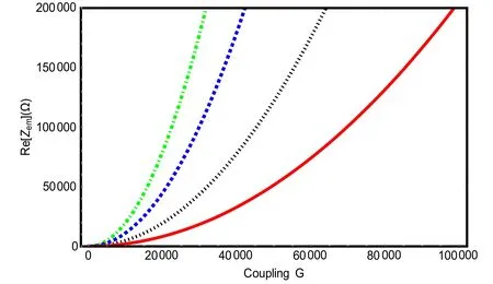
Figure 4.The real part of the reactance diagram of the capacitor: the red continuous diagram belongs to the phenomenological dissipation(Гm=2π*20 Hz)and the{green dotted-dashed,blue dashed,black dotted}plots are associated with R={13,23,53}Ω wherein the CK dissipation has been used.Also,we considered the resonance condition (Ωm=Ω) for typical parameters m=36 ng,Ω m=2π*700 kHz,Cm (x=0)=0.5 pF.

where we have defined

In [5] based on phenomenological dissipation,with specified parameters the efficiency has been obtained at about 48%.However,based on the above relations,and with the same parameters,in the CK approach the efficiency of the system depends on the power supply voltage (see figure 5).

As is seen from figure 5,with increasingR,the efficiency of the system decreases,and maximum efficiency is obtained at higher supply voltages.In addition,the variation ofγ(membrane damping) does not have a critical effect on the efficiency of the system.

5.Concluding remarks

In summary,we have considered an electro-optomechanical system with CK dissipation by which we aimed to check (i)mechanically induced transparency,(ii)created phase shift in the optical field by moving the membrane,(iii) electromechanical impedance,and(iv)system efficiency.In order to compare the dissipation effects using the CK Hamiltonian approach and the previously phenomenological method,we have used the same parameters as in [5].In general,logical,analytical,and reliable results are observed in the performance of the system under the influence of the dissipation with the Hamiltonian CK compared with the phenomenological method.

In more detail,with increasingRthe following realizations can be observed:

i.The inductive transparency phenomenon (at low coupling values) and the ratioδVc/δVs(at different coupling coefficients) decrease,except at the coupling coefficientG=50 kV m−1wherein this ratio strongly increases.

ii.The displacement of the membrane is reduced and its maximum occurs at lower supply voltages.Also,the influence of the dissipative electromechanical subsystem on the membrane displacement is much higher than on the dissipative optomechanical subsystem,such that the latter can be ignored compared to the former.

iii.In all cases,system impedance decreases at higher coupling coefficients.

iv.The system efficiency is reduced,and its maximum can be achieved at higher supply voltages.Also,changingγ(membrane damping) does not have a significant effect on the system efficiency.

To compare the above results with the phenomenological method,it should be stated that the main source of dissipation has arisen from the optomechanical subsystem.Therefore,either by reducing the mechanical damping (at low coupling coefficients) or by increasing the coupling coefficient (by keeping the mechanical damping at a constant value),the impedance of the system can be increased.The imaginary reactance of the capacitor in both the dissipation methods,i.e.,CK or phenomenological dissipation methods remains constant.

As an important advantage of our approach,we can refer to the fact that by using the CK Hamiltonian,the performance of the system behavior via the influence of dissipation components can be more easily controlled.This means that the dissipation sources in the CK Hamiltonian approach are more controllable than those of the phenomenological approach.

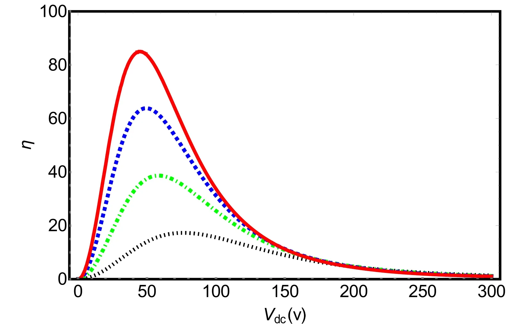
Figure 5.System efficiency diagram in terms of electrical supply voltage changes: The red continuous diagram refers to phenomenological dissipation (ГLC=2π*5.5 kHz,Гm=2π*2 Hz) and the {blue dashed,green dotted-dashed,black dotted} plots are associated with R={5.5,6.5,8.5} wherein the CK dissipation has been used.The chosen parameters are as m=28 ng,γ=0.5,λ=1064 nm,a=55,Ω m=Ω=2π*690 kHz,L=1 mH,Cm (x=0)=0.5 pF,Vs=10 nV,G=50 kV m−1.

Acknowledgments

The authors would like to thank Dr Anders Simonsen from Niels Bohr Institute,University of Copenhagen for useful discussions.