Rogue Waves and Lump Solitons of the(3+1)-Dimensional Generalized B-type Kadomtsev–Petviashvili Equation for Water Waves∗

Yan Sun(孙岩),Bo Tian(田播), Lei Liu(刘磊),Han-Peng Chai(柴汉鹏),and Yu-Qiang Yuan(袁玉强)

State Key Laboratory of Information Photonics and Optical Communications,and School of Science,Beijing University of Posts and Telecommunications,Beijing 100876,China

1 Introduction

Rogue waves,initially termed to describe the extreme wave events that emerge in the deep ocean,[1−2]have been concerned both in experimental observations and theoretical predictions.[3−4]Generally,rogue waves have been observed to appear from nowhere and disappear without a trace.[5]Rogue-wave solutions have been thought to be a kind of the rational solution localized in both space and time,which has been reported in fluid mechanics,[6−7]capillary-wave physics[8−9]and nonlinear optics.[10−12]Lump-soliton solutions,another kind of the rational solutions,have been localized in all directions in the space.[13]Besides,since there is no relation between the amplitude and width of a lump soliton,the pro file of the lump soliton has been diverse.[13]Lump-soliton solutions have been proved to support the meromorphic structures which can guarantee their stability,while rogue-wave solutions,not.[14]Lump soliton solutions have been seen to describe the nonlinear patterns in a plasma,[15]optic medium[16]and shallow water with the dominated surface tension.[17]There have been some methods for deriving the analytic rogue wave solutions and lump soliton solutions,such as the Darboux transformation,[18−19]Darboux dressing technique,[20]B¨acklund transformations,[21]and Kadomtsev–Petviashvili(KP)hierarchy reduction.[22−26]

Researchers have imposed an extra condition between the Lax operator and its adjoint of the KP hierarchy so that the KP hierarchy of B type have been obtained.[27−28]In the KP hierarchy of B type,researchers have focused their attention on the generalized(3+1)-dimensional B-type KP(BKP)equation for water waves,[28−31]

whereuis a real function of the scaled spatial coordinatesx,y,zand temporal coordinatet.The first-order lump solutions of Eq.(1)have been derived.[29]Pfaffian and multi-wave solutions of Eq.(1)have been studied.[28,30]Forming linear subspaces of solutions,resonant solitons of Eq.(1)have appeared.[31]

To our knowledge,the higher-order,multiple rogue waves and lump solitons of Eq.(1)have not been studied by means of the symbolic computation and Hirota method,[32−37]and KP hierarchy reduction.[22−26]In this paper,by virtue of the Hirota method and KP hierarchy reduction,rogue wave and lump soliton solutions in terms of the Gramian of Eq.(1)will be given in Sec.2.Discussions on the rogue waves and lump solitons will be presented in Sec.3.Section 4 will be our conclusions.

2 Rogue Wave and Lump Soliton Solutions in Terms of the Gramian of Eq.(1)

Under the dependent variable transformation

Eq.(1)can be transformed into the following bilinear form:[29]

wherefis a real function ofx,y,zandt,Dx,Dy,Dz,andDtare the bilinear differential operators de fined by[32]

withFas a function ofx,y,z,andt,Gas a function of the formal variablesx′,y′,z′,andt′,χ1,χ2,χ3,andχ4being the non-negative integers.

In order to obtain the rogue waves and lump solitons,we start with the Gramian expression of the KP hierarchy[26−27]and present the rogue wave and lump soliton solutions in terms of the Gramian of Eq.(1)in the following Theorem 1.

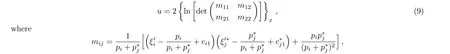
Theorem 1Equation(1)has the rogue wave and lump soliton solutions in terms of the Gramian,

where˜pj’s are the complex variables,“∗”means the complex conjugate,i,j,Nandnj’s are the positive integers,pj’s andcjl’s are the complex constants.The proof of Theorem 1 is given in the Appendix.We can normalizecj0=1 by a scaling off,and hereafter setcj0=1 without loss of generality.

3 Rogue Waves and Lump Solitons of Eq.(1)

3.1 The First-Order Rogue Waves and Lump Solitons

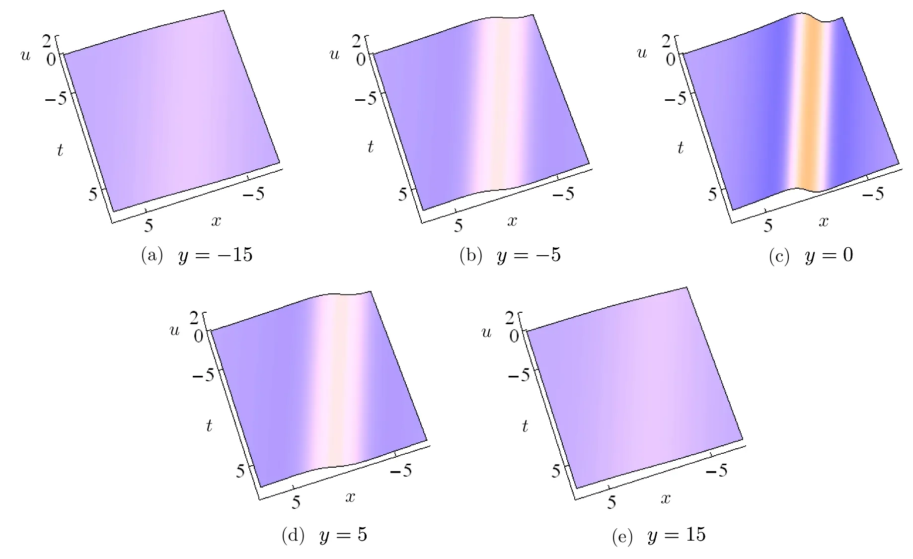
Fig.1 The first-order rogue wave via Solutions(8)at z=0 with p1=0.25 and c11=0.

The first-order rogue wave and lump soliton solutions are given withN=1 andn1=1,

From Solutions(8),p1cannot be purely imaginary since the denominator offcannot be zero.

Figures 1 present the first-order line rogue wave.The rogue wave approaches the constant background on the(x,t)plane when|y|increases,but the amplitude of the rogue wave reaches the maximum wheny=0,which is distinctly different from that of the moving line solitary waves.Shown in Figs.2 is a first-order lump soliton.The lump soliton is localized in all directions with both upper and down humps and it propagates stably on the(x,t)plane.

Fig.2 The first-order lump soliton via Solutions(8)at z=0 with p1=0.5−0.4i and c11=0.

3.2 The Multiple Rogue Waves and Lump Solitons

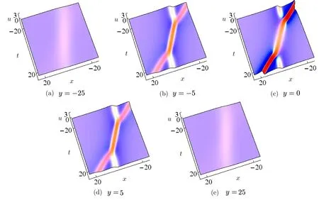
Fig.3 The two rogue waves via Solutions(9)at z=0 with p1=−0.2,p2=0.4 and c11=c21=0.

To derive the multiple rogue waves and lump solitons,we considerN=2 andn1=1 from Solutions(4)as

ξ′j’s are given in expression(7).

As seen in Figs.3,when|y|is large enough,the two rogue waves approach the constant background.Otherwise,the two rogue waves arise from the constant background and interaction with each other.Especially,wheny→0,their interaction region acquires the highest amplitude.With large|y|,interaction fades and two rogue waves begin to disappear.

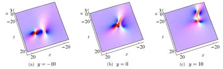
Fig.4 The two lump solitons via Solutions(9)at z=0 with p1=0.3+0.2i,p2=0.4+0.3i and c11=c21=0.

Fig.5 The three rogue waves and lump solitons at z=0 with(a)p1=0.4,p2=−0.3 and p3=0.15;(b)p1=−0.3−0.3i,p2=0.4−0.4i and p3=0.5+0.5i.

Figures 4 demonstrate the two lump solitons,whose interaction is different from that in Figs.3.As shown in Figs.4,the two lump solitons propagate with different amplitudes and velocities.They interact with each other whent=0.Soon after that,they separate from each other and maintain their original states.We can observe that during the process of interaction,shapes of the lump solitons do not change.Thus,the interaction is elastic.

For the largerN,the multiple rogue waves and lump solitons have qualitatively similar behaviors,except that more rogue waves and lump solitons arise and interact with one another,and more complicated wavefronts form in the interaction region.We illustrateN=3 as an example in Figs.5.

3.3 The Higher-Order Rogue Waves and Lump Solitons

The higher-order rogue wave and lump soliton solutions can be obtained withN=1 andn1＞1 in Solutions(4).In order to derive second-order rogue waves and lump solitons,we can setni=2 from Solutions(4)as

Here we setc11=0.

Shown in Figs.6 are the second-order rogue waves.Comparing Figs.6 with Figs.1,we can see that the second-order rogue waves can be treated as a superposition of two first-order rogue waves.Unlike the oblique interaction in Figs.3,we can observe in Figs.6 that the two waves first interact obliquely and then fuse to one wave.Soon after that,the two waves recover their original states.

As shown in Figs.7,the second-order lump solitons propagate with the different velocities,while they also merge wheny=0.Soon after that,they separate from each other.We can observe that during the interaction,shapes and velocities of the lump solitons change,unlike the two lump solitons in Figs.4.Thus,the interaction is inelastic.

Fig.6 The second-order rogue waves via Solutions(10)at z=0 with p1=−0.3 and c12=0.

Fig.7 The second-order lump solitons via Solutions(10)at z=0 with p1=0.286−0.3i and c12=0.

4 Conclusions

In this paper,we have investigated a(3+1)-dimensional generalized BKP equation for water waves,i.e.,Eq.(1).Based on the Hirota method and KP hierarchy reduction,rogue wave and lump soliton solutions have been given in the Gramian,i.e.,Solutions(4).According to Solutions(4),we have derived the first-order,higher-order and multiple rogue waves and lump solitons.In Figs.1,we have observed that the first-order rogue waves are the line rogue waves which arise from the constant background and then disappear into the constant background again on the(x,t)plane.Localized in all directions with both upper and down humps,lump solitons propagating stably on the(x,t)plane have been presented in Figs.2.In Figs.3,two rogue waves have been seen to describe the interaction between the two first-order rogue waves.Unlike the two rogue waves in Figs.3,localized two lump solitons have been seen to remain stable during the interaction,as seen in Figs.4.Figures 5 have shown the three rogue waves and lump solitons,of which the behaviors are similar to those of the two rogue waves and lump solitons.The higher-order rogue waves have been presented in Figs.6 and 7,as the superpositions of the first-order rogue waves as well as higher-order lump solitons.Comparing Figs.6 with Figs.3,we have observed that the two waves fuse to one wave.Comparing Figs.7 with Figs.4,we have observed that the interaction between the second-order lump solitons is inelastic.

Appendix

We will prove Theorem 1 in Sec.2.

where“∂” means the partial derivative,i,jandnare the positive integers.Then,the determinant

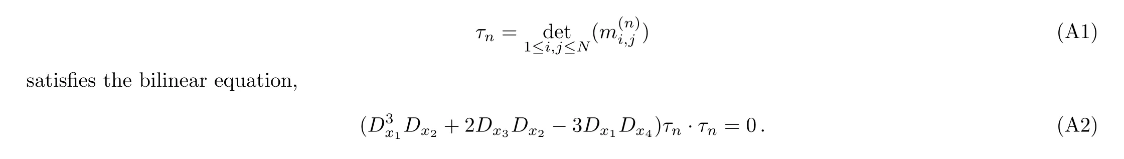
ProofBased on the Gramian technique,[32]we can verify that the derivatives and shifts of theτfunction(A1)are expressed by the bordered determinants as follows:

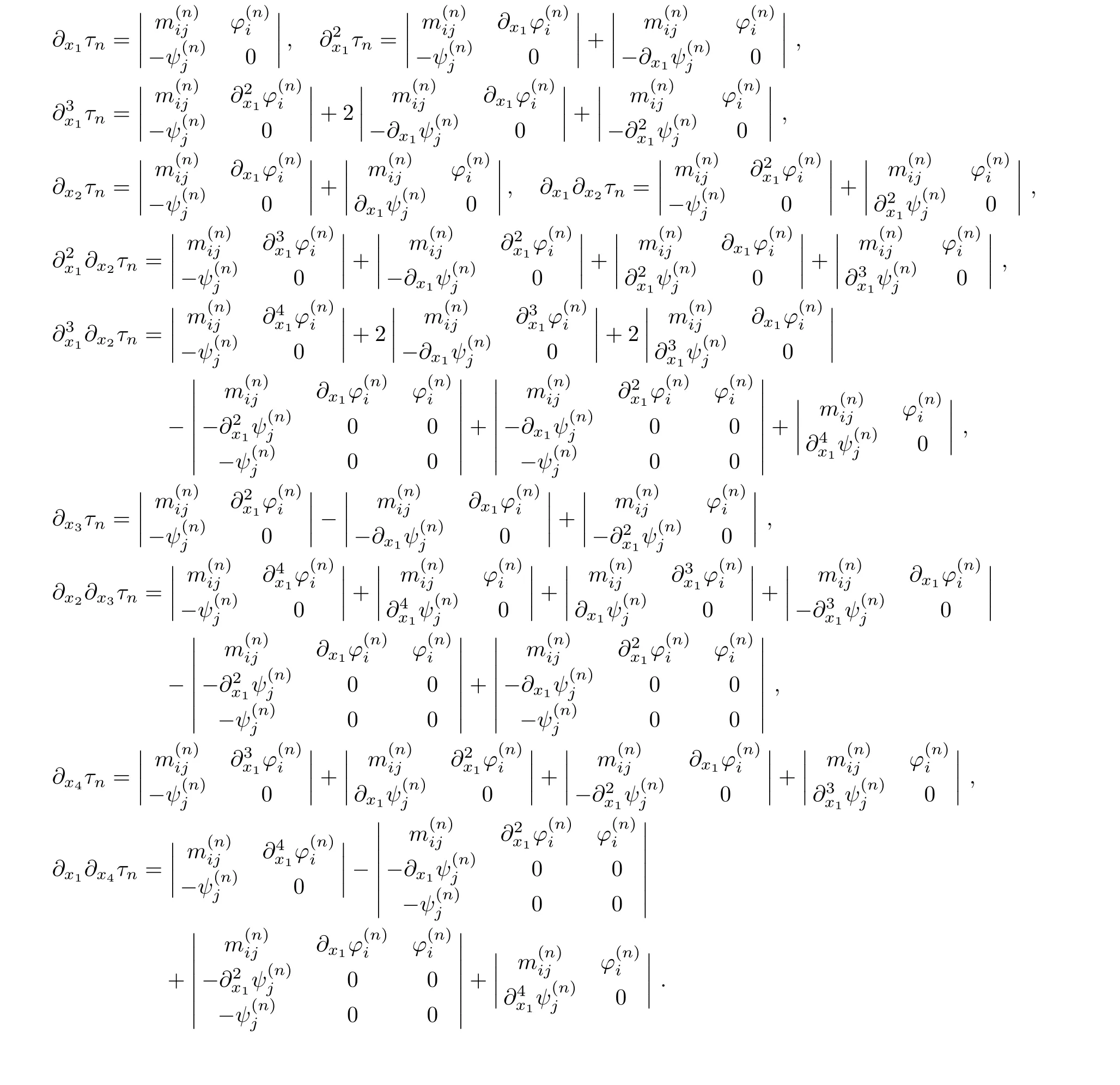
we can obtain thatτfunction(A1)satis fies Expression(A2).The proof is completed.

Next we use this Lemma to proof Theorem 1.

withpi’s,qj’s,cik’s,djl’s being complex constants,˜pi’s,˜qj’s being complex variables andi,j,nj’s,Nbeing positive integers.Due to the gauge freedom ofτn,we can see that

gives the same solution as Expression(A3).

In order to study the rogue wave and lump soliton solutions for Eq.(1),we setτ0=f,apply the transformation of independent variablesx1=−x,x2=iy,x3=2t,x4=izand take the parameter constraintsqj=p∗j,djl=c∗jl.Then we haveη′j=ξ′∗j.

Thus,Expression(A2)can be transformed into Bilinear Form(3).Under Transformation(2),Solutions(4)of the Eq.(1)given in Theorem 1 can be obtained from Expression(A2).Thus Theorem 1 has been proved. □

[1]C.Kharif and E.Pelinovsky,Eur.J.Mech.B Fluids 22 603(2003).

[2]E.Pelinovsky and C.Kharif,Extreme Ocean Waves,Springer,Berlin(2008).

[3]B.Kibler,J.Fatome,C.Finot,et al.,Nat.Phys.6(2010)790.

[4]J.M.Soto-Crespo,P.Grelu,and N.Akhmediev,Phys.Rev.E 84(2011)016604.

[5]N.Akhmediev,A.Ankiewicz,and M.Taki,Phys.Lett.A 373(2009)675.

[6]H.Bailung,S.K.Sharma,and Y.Nakamura,Phys.Rev.Lett.107(2011)814.

[7]H.X.Jia,Y.J.Liu,and Y.N.Wang,Z.Naturforsch.A 27(2015)71.

[8]M.Shats,H.Punzmann,and H.Xia,Phys.Rev.Lett.104(2010)104503.

[9]H.Xia,T.Maimbourg,H.Punzmann,and M.Shats,Phys.Rev.Lett.109(2012)114502.

[10]D.R.Solli,C.Ropers,P.Koonath,and B.Jalali,Nature(London)450(2007)1054.

[11]D.W.Zuo,Y.T.Gao,L.Xue,and Y.J.Feng,Opt.Quant.Electron.48(2016)1.

[12]S.L.Jia,Y.T.Gao,C.Zhao,Z.Z.Lan,and Y.J.Feng,Eur.Phys.J.Plus 132(2017)255.

[13]H.C.Ma and A.P.Deng,Commun.Theor.Phys.65(2016)546.

[14]J.Villarroel,J.Prada,and P.G.Estevez,Stud.Appl.Math.122(2009)395.

[15]V.I.Petviashvili and O.V.Pokhotelov,Solitary Waves in Plasmas and in the Atmosphere,Energoatomizdat,Moscow(1989).

[16]D.E.Pelinovsky,Y.A.Stepanyants,and Y.S.Kivshar,Phys.Rev.E 51(1995)5016.

[17]E.Falcon,C.Laroche,and S.Fauve,Phys.Rev.Lett.89(2002)204501.

[18]V.B.Matveev and M.A.Salle,Darboux Transformations and Soliton,Springer,Berlin(1991).

[19]Q.M.Huang,Y.T.Gao,and Lei Hu,Appl.Math.Lett.75(2018)135.

[20]O.C.Wright,Chaos,Solitons and Fractals 33(2007)374.

[21]X.Y.Gao,Appl.Math.Lett.73(2017)143.

[22]Y.Ohta and J.Yang,Phys.Rev.E 86(2012)036604.

[23]Y.Ohta and J.Yang,Proc.R.Soc.A 468(2012)1716.

[24]Y.Zhang,Y.B.Sun,and W.Xiang,Appl.Math.Comput.263(2015)204.

[25]M.Sato,RIMS Kokyuroku 439(1981)30.

[26]M.Jimbo and T.Miwapubl,RIMS Kokyuroku 19(1983)93.

[27]E.Date,M.Jimbo,M.Kashiwara,and T.Miwa,Physica D 4(1982)343.

[28]M.G.Asaad and W.X.Ma,Appl.Math.Comput.218(2012)5524.

[29]W.X.Ma,Z.Y.Qin,and X.L¨u,Nonlinear Dyn.84(2016)923.

[30]W.X.Ma and Z.N.Zhu,Appl.Math.Comput.218(2012)11871.

[31]W.X.Ma and E.G.Fan,Comput.Math.Appl.61(2011)950.

[32]R.Hirota,The Direct Method in Soliton Theory,Cambridge University Press,Cambridge(2004).

[33]Z.Z.Lan,Y.T.Gao,J.W.Yang,C.Q.Su,and B.Q.Mao,Commun.Nonlinear Sci.Numer.Simulat.44(2016)360.

[34]X.Y.Gao,Ocean Eng.96(2015)245.

[35]J.J.Su,Y.T.Gao,and S.L.Jia,Commun.Nonlinear Sci.Numer.Simulat.50(2017)128.

[36]G.F.Deng and Y.T.Gao,Eur.Phys.J.Plus 132(2017)255;G.F.Deng and Y.T.Gao,Superlattices Microstruct.109(2017)345;Q.M.Huang,Y.T.Gao,S.L.Jia,and G.F.Deng,Nonlinear Dyn.87(2017)2529.

[37]T.T.Jia,Y.Z.Chai,and H.Q.Hao,Superlattices Microstruct.105(2017)172.