A cautionary note on decadal sea level pressure predictions from GCMs

Stefan LIESS*,Peter K.SNYDER,Arjun KUMAR,Vipin KUMAR

a Department of Earth Sciences,University of Minnesota,Minneapolis MN 55455,USA

b Department of Soil,Water,and Climate,University of Minnesota,St.Paul MN 55108,USA

c Computer Science&Engineering,University of Minnesota,Minneapolis MN 55455,USA

1.Introduction

Observational analyses have documented distinct patterns of the Atlantic Ocean variability with decadal(8-12 years)and multidecadal(30-80 years)time scales(Delworth et al.,2007).General circulation models(GCMs)from the third and fifth phases of Coupled Model Intercomparison Project(CMIP)have succeeded in capturing some aspects of this observed variability(Medhaug and Furevik,2011;Zhang and Wang,2013).The resulting decadal predictability remains in fluenced by the initial conditions from slow components of the climate system(Collins,2007;Pohlmann et al.,2009).Some techniques to improve decadal predictions include biascorrection of initial conditions(Laepple et al.,2008).Keenlyside et al.(2008)found increased prediction skill after initializing the ECHAM5/MPI-OM GCM with sea surface temperatures(SST)that were nudged to observed SSTs.GCM simulations show that changes in SST and sea ice variability can be related to the Atlantic Meridional Overturning Circulation(AMOC)(Mahajan et al.,2011a,2011b;Zhang and Wang,2013),and the strength is potentially predictable for up to a decade,with skill varying among models(Matei et al.,2012;Pohlmann et al.,2009).

Decadal trends in Arctic sea level pressure(SLP)have previously been noted by Walsh et al.(1996),and Latif et al.(2000)have investigated the predictability of decadal wintertime North Atlantic SLP variations.Latif et al.(2000)found considerable evidence that these SLP variations on timescales of several years to decades may be predictable in their analysis of the ECHAM4 model,which is a predecessor to the atmospheric version of the CMIP3 model ECHAM5/MPI-OM.They found that the simulated North Atlantic Oscillation(NAO)is significantly correlated at 0.32 with observations,and smoothing both time series with canonical correlation analysis reveals a correlation of 0.65.In general,GCMs are known to exhibit more zonally symmetric annular modes than observations(Gerber et al.,2008,2010;Xin et al.,2008).Thus,zonally averaged trends are considered appropriate for capturing the variations in simulated annular mode activity.

Because multidecadal oscillations of geopotential height and temperature can stretch over multiple ocean basins(Lee and Hsu,2013),it is tempting to analyze if large-scale SLP changes over these larger zones can be predicted on the decadal scale,similar to the previously discussed results by Latif et al.(2000).The dependence of annual mean SLP on latitudinal zones and seasonal variation has been previously analyzed by Trenberth(1981).Correlations between northern and southern annular modes are linked to Madden-Julian oscillation(MJO)activity,with lags in daily data being smoothed in the monthly averages used in the present study(Flatau and Kim,2013).

The Northern Annular Mode(NAM)exhibits the strongest variability during the December-January-February(DJF)season(Gillett and Fyfe,2013;Hurrell,1995,1996),whereas the Southern Annular Mode(SAM)variability remains similar for all seasons(Trenberth,1991)and also shows a strong axisymmetric pattern around the South Pole in DJF(Simmonds,2015).Poleward propagating Rossby waves can provide symmetric patterns around the equator(Flatau and Kim,2013;L'Heureux and Thompson,2006;Liess et al.,2014),prompting a combined analysis of SLP trends over both hemispheres.SLP variability is relatively low over low latitudes(Gillett and Stott,2009).Gillett et al.(2005,2003)state that both positive and negative trends are up to one order of magnitude lower in GCM ensemble simulations compared to observations because simulations with opposing phases of large-scale oscillations are averaged to form the ensemble mean.Thus,ensemble simulations that smooth out the internal variability indicate the portion of external variability.It is assumed here that individual GCM simulations with trends similar to observations also exhibit a similar combination of trends from internal and external forcings.Systematic model errors are thus neglected in this study.

However,large-scale relations can be well represented in GCMs(Casado and Pastor,2012;Handorf and Dethloff,2012;Pastor and Casado,2012;Stoner et al.,2009),thus justifying the circumglobal approach in this study.Circumglobal Rossby wave trains in the Northern Hemisphere have been identified for boreal summer(Ding and Wang,2005;Schubert et al.,2011;Teng et al.,2013)and winter(Branstator,2002;Liess et al.,2017).Here we analyze the global SLP field because it is closely linked to near-surface winds and other climate processes that need to be predicted for policymakers.Although the SLP field is noisier than mid-and uppertropospheric geopotential height fields,SLP trends are important indicators for changing weather and climate patterns(Gillett et al.,2013).The role of stratospheric and other nonoceanic drivers in decadal climate predictability has been discussed in detail by Bellucci et al.(2015).

Gillett et al.(2005,2003)and Miller et al.(2006)have associated a decrease in high-latitude SLP with anthropogenically in fluenced increase in greenhouse gases(GHG)and ozone depleting substances with the latter being primarily important in the Southern Hemisphere forcing(Arblaster and Meehl,2006;Gillett and Fyfe,2013;Gillett and Thompson,2003;Simmonds,2015;Wilmes et al.,2012).This negative SLP trend over high-latitudes is accompanied by an SLP increase over low and mid-latitude regions,resembling the annular modes.These long-term externally forced trends are superimposed by internal low frequencies in the annular modes that can provide varying SLP trends on the decadal time scale.This combination of externally forced variability and the internal low-frequency variability that comprises the decadal climate time scale is most relevant for policymakers and is therefore the focus of this study.

The time frame since 1979,when satellite data became widely available,or subsets of time frames within this recent period have been widely used for observational studies(Trenberth et al.,2005)and CMIP3 model intercomparison studies(e.g.,Karpechko et al.,2009;Pincus et al.,2008).Although external forcing is similar for all 20th century CMIP3 simulations,internal Atlantic Multidecadal Oscillation(AMO)and Pacific Decadal Oscillation(PDO)phases have been found to be quite different(Meehl et al.,2009).Even the more recent decadal CMIP5 simulations with observed initial conditions can produce a variety of AMO and PDO phases,and spatial AMO representation shows both improvements and deterioration from CMIP3 to CMIP5 depending on the model(Ruiz-Barradas et al.,2013).However,in general,AMOC and AMO simulations have been improved in CMIP5 compared to CMIP3(Zhang and Wang,2013).The objective of this paper is to discuss the reliability of decadal predictions and to point out a spurious result that puts artificial con fidence in widely used CMIP3 predictions since 1979.This con fidence is not corroborated by other time frames or more recent CMIP5 predictions.

Section 2 of this paper introduces a simple method that ranks CMIP3 and CMIP5 ensemble members by their representation of different phases within the multidecadal SLP variability and attempts to improve predictions of large-scale SLP trends.Results of the analysis are described in Section 3.Section 4 provides a summary and a conclusion.

2.Methods and data

This study uses seasonal mean HadSLP2 observations(Allan and Ansell,2006)for the DJF seasons from 1957 to 2011 to determine relationships between decadal trends for thefive high(80°S-50°S and 50°N-80°N),mid(50°S-20°S and 20°N-50°N),and low(20°S-20°N)latitude zones as identified by their deviation from the average SLP.Fig.1 shows the average SLP during DJF for the widely used 1979-2000 period.Also shown on the right is the zonal mean value in comparison to the 1013.25 hPa global mean value based on the USA standard atmosphere(NASA,1976),which shows that the five regions mentioned above can be distinguished by their deviation from the global mean.The southernmost region shows a strong negative deviation,the two midlatitudinal zones show moderate positive deviations,and the northernmost and tropical zones show virtually no deviations.The long-term trend pattern shown by Gillett and Stott(2009)corroborates these distinctions and shows that long-term changes enhance most of the deviations from the global mean.However,previous research by Walsh et al.(1996)and Latif et al.(2000)shows that there is decadal variability within this long-term trend.

Decadal climate variability in mid-and high-latitudes is re flected in modifications of the southern and northern annular modes.Thus,the southernmost two zones in our study correspond roughly to the two ends of the SAM,and we select the northernmost two zones to capture trends in the NAM.

We calculate linear trends of SLP for 1979-2000(referred to as initialization period)separately for high-,mid-,and lowlatitude zones,and rank CMIP3 model simulations by their ability to match observed trends.For a limited subset of CMIP3 GCMs,we also show predictions that seem to be improved during the 2001-2011 decade(referred to as hindcast period)when excluding members from the multimodel ensemble(MME)that would produce initial conditions from opposing phases during the prior spin-up period.

Here,we analyze 38 individual ensemble members from nine CMIP3 coupled atmosphere-ocean GCMs.Each GCM provides at least three ensemble members with continuous simulations for the 20th century as well as the A1B scenario(Nakicenovic et al.,2000)after 2000.Ensembles for each GCM use slightly different initial conditions and are thus different realizations of simulated climate characteristics.We compare these 38 CMIP3 ensemble members to 38 ensemble members from CMIP5 decadal simulations,which are successors of the CMIP3 models,where available.The CMIP5 models use observed external forcing based on the RCP4.5 scenario(van Vuuren et al.,2011)after 2005.

Fig.1.Global SLP field during DJF for 1979-2000 from HadSLP2 observations.The right panel shows zonal mean values in comparison to the global mean value of 1013.25 hPa(vertical line).

Table 1List of GCMs used in this study with number of ensemble members in parentheses.

The CMIP3 and CMIP5 GCMs as well as the number of ensembles for each GCM are listed in Table 1.However,it should be noted that although many studies compared CMIP3 results to observations starting with the satellite era in 1979,decadal CMIP5 simulations start at the first year of every decade,in this case in 1981.In order to compensate for this discrepancy,our study utilizes different time frames for CMIP3 and CMIP5 simulations that remain within 10%of each other's time frames and overlap over 90%of the time.The CMIP3 analysis uses the 1979-2000 initialization and 2001-2011 hindcast periods,whereas the CMIP5 analysis comprises of the 1981-2000 initialization and 2001-2010 hindcast periods.Thus,the length of the hindcast period is exactly 50%of the initialization period in both analyses.The time period is cut in half from the initialization period to the hindcast experiments,because forecasting skills of atmospheric oscillations are often less than one cycle(i.e.information about a 22-year period might be required for an 11-year prediction),and predictability is suggested to decrease strongly after one decade(Kim et al.,2012;Pohlmann et al.,2009).

For an estimate of model skill,we analyze individual ensemble members and compare the results to observed SLP trends over the zones defined above.The trend analysis is performed with linear least squares regression.The statistical significance of the trend is calculated from the ratio between the estimated trend and its standard error(Santer et al.,2000).

In addition to testing the significance of individual trends,we test if individual ensemble members of a given GCM retain large-scale information from the initialization period for trends during the following decade,the hindcast period.For this,we rank ensemble members by their performances during the initialization and hindcast periods(lower rank is better and indicates less difference between observed and simulated trend).We then use linear regression to test for significant relationships between the ranks of the initialization and hindcast periods.Finally,we calculate mean trends and their standard deviations separately for each GCM before calculating the overall mean and standard deviation so that systematic errors of GCMs with many ensemble members are not dominating the overall results.Thus, first the trends of each ensemble member of each model are averaged,and next the model mean trends are averaged into a multi-model mean trend,similar to the MME calculation described in van Oldenborgh et al.(2012).Eq.(1)defines the overall standard deviation,which is adjusted to accommodate the different means μ and standard deviations σ for each modeljwith μ（T）being the multi-model mean of all trendsT.

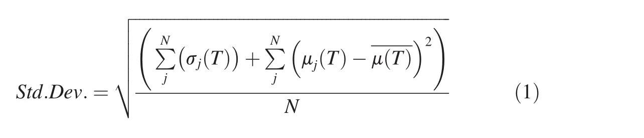
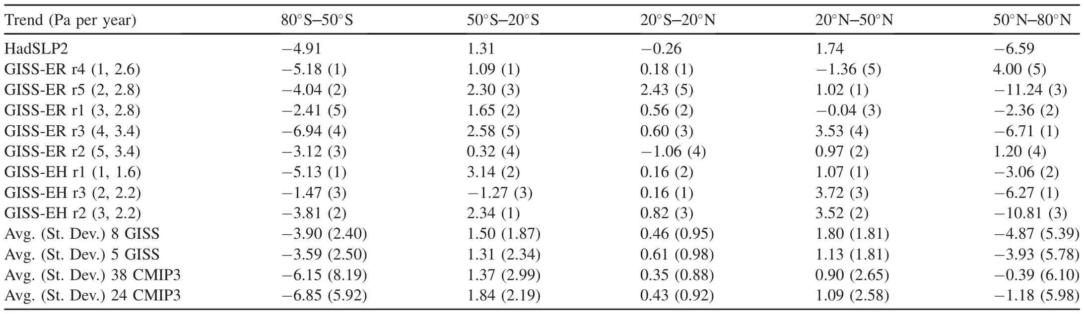
Table 2Area averaged SLP trends in 1979-2000 for HadSLP2 observations and the two best performing CMIP3 GCMs.Numbers in parenthesis indicate the rank of each ensemble member within each GCM.The total ranks also include the average rank value over the five zones.The last four rows show average and standard deviation for the GISS and CMIP3 MMEs using all ensemble members and all except the lowest performing ensemble members,respectively.

3.Analysis of SLP trends

3.1.SLP trends in initialization periods

Table 2 shows area averaged 22-year SLP trends during DJF in 1979-2000 for HadSLP2 observations and the CMIP3 versions of the GISS-ER and GISS-EH models,which provide ensemble members with trends close to the observed.1See Table A1 in https://www.cs.umn.edu/sites/cs.umn.edu/ files/tech_reports/18-002.pdf.Also listed are the average trends and their standard deviations for all eight GISS ensemble members(also known as runs,abbreviated as rnin this study,withnreferring to the ensemble number),and the average trends and their standard deviations for all GISS ensemble members except the two worst performing members(one if only three members exist).This step is motivated by the attempt to reduce the ensemble prediction error when members with poor performance during the initialization period are excluded from the MME prediction.The bottom two rows in Table 2 show results for all 38 ensemble members from the nine CMIP3 GCMs,and for all except 14 poorly performing ensemble members.From the nine available CCSM3 ensemble members,only seven are used,since r4 and r8 do not continue with A1B projections.The remaining CCSM3 ensemble members are thus ranked from 1 to 7.

The ensemble members from each model are sorted by average rank over all the five zones that are listed in Table 2 with each zone being equally weighted for the overall average,despite the higher latitude zones being smaller in area than lower latitude zones.Here it is suggested that higher latitude zones have a stronger signal in decadal SLP variability,therefore they receive stronger weights per area.If two ensemble members of the same GCM have the same average rank,such as r2 and r3 in GISS-ER,which both have an average rank of 3.4(see Table 2),then the ensemble member with the larger spread of ranks over the five zones is considered to be favorable for predictions.In this case,r3 is ranked better because of the wider spread from 1 to 5 compared to r2 with a narrower spread from 2 to 4.A wider spread is considered to be favorable for predictions,because it increases the chance that the spread interval includes trends close to observations for some zones.If two ensembles have the same spread,a conservative approach is taken that assumes the ranks between initialization and hindcast do not match.In Table 2,the different models are sorted with the best model during initialization appearing first.For this rank,the lowest detected SLP errors for each GCM and each zone are averaged over the five zones.2See Table A1 in https://www.cs.umn.edu/sites/cs.umn.edu/ files/tech_reports/18-002.pdf.

After excluding the lowest performing ensemble members from the GISS-only MME,the average trend for 1979-2000 improves over the Southern Hemisphere mid-latitudes,but slightly deteriorates over all other four zones.For the MME for all nine GCMs,the average trend for this period improves over the Northern Hemisphere but deteriorates over the Southern Hemisphere and the tropics.In general,the observed trends remain within one standard deviation of all averaged trends,apart from the Arctic zone,where the MME for all nine GCMs does not capture the strong negative trend.However,excluding poorly performing ensemble members decreases this error so that the strong trend over the Arctic zone is included within one standard deviation of the MME trend.As expected for fewer ensemble members,the standard deviation decreases in four out of five zones for the MME of all nine GCMs,which in the present case reduces the MME uncertainty.Based on these results with commonly studied GCMs,one might assume that both MME error and standard deviation can be decreased when poor performing ensemble members are excluded for decadal predictions.

To further illustrate the selection process during the 1979-2000 period,the observed trends(Fig.2a)are compared to the excluded ensemble members of GFDL-CM2.1(Fig.2b)and ECHAM5/MPI-OM(Fig.2c-d).The ensemble members in Fig.2 fail to simulate the strength of the negative trend in the northern high-latitudes and only ECHAM5/MPI-OM r4 captures the slight positive trend in the northern mid-latitudes.None of these ensemble members produce an increase in SLP over the southern mid-latitudes,and GFDL-CM2.1 r1 and ECHAM5/MPI-OM r4 also do not capture the simultaneous decrease over southern high-latitudes indicating the strengthening of SAM during this time period.The trend over the tropics is only slightly negative in HadSLP2 and stronger negative in these ensemble members,but SLP variability is relatively low in the tropics(Gillett and Stott,2009),and thus not discussed in detail here.

The remaining ensemble members of these two models produce more realistic trend patterns(Fig.3).For example,these ensemble members simulate the increased strength in SAM as shown by the negative(positive)trend over high-(mid-)latitudes.However,only GFDL-CM2.1 r2 simulates a negative trend in northern high-latitudes whereas other ensemble members produce an erroneous positive trend,and all ECHAM5/MPI-OM ensemble members apart from r4,which has been excluded because of poor performance over the Southern Hemisphere,generate an erroneous negative trend in northern mid-latitudes.These erroneous trends explain why these two models are ranked low,only followed by MIROC3.2(medres),which produces overly strong trends over the Southern Hemisphere.3See Table A1 in https://www.cs.umn.edu/sites/cs.umn.edu/ files/tech_reports/18-002.pdf.

Decadal CMIP5 ensemble members are initialized with initial conditions re flecting the conditions of a particular year and generally cover a 30-year simulation period.The 1980 decadal experiment starts on 1st January 1981,and 1981-2000 is selected here as initialization period with the remaining ten years being used as hindcast period.The ranking of CCSM4 ensemble members results from the model's performance over the Northern Hemisphere,whereas CanCM4,MIROC5 and MPI-ESM-LR are mostly ranked related to their Southern Hemisphere performance.Ranking for the other three models(FGOALS-g2,MIROC4h,and MRI-CGCM3) results from performance over both hemispheres.

Table 3 shows HadSLP2 trends and average trends for all 38 ensemble members from all seven CMIP5 models and the best 20 ensemble members from all seven CMIP5 models.Trends were calculated first for each model and then averaged over the number of models.As in CMIP3(see Table 2),average trends over all seven CMIP5 GCMs were improved over the two northernmost zones when the worst performing ensemble members are excluded,but results over the other three zones deteriorated.In general,the observed trends remain within one standard deviation of all averaged trends,apart from the Antarctic zone,where the MME produces a positive trend with a standard deviation outside of the observations,after the worst performing ensemble members are excluded.These results indicate no significant improvements when the worst performing ensemble members are excluded.

Fig.2.SLP trends during DJF for 1979-2000 from(a)HadSLP2 observations and(b-d)individual GFDL-CM2.1 and ECHAM5/MPI-OM ensemble members that are found to have zonal trends different from HadSLP2.Black dots indicate significant trends at the 95%con fidence interval.

3.2.SLP trends in hindcast periods

In the HadSLP2 observations,the 11-year SLP trend for 2001-2011 showsastrong negativesignaloverthehigh-latitude Southern Hemisphere and a slightly positive trend overthe highlatitude Northern Hemisphere(Table 4),explaining the different characteristics of polar amplification over both hemispheres during DJF(Simmonds,2015).

It should be noted that the GFDL-CM2.1 A1B ensemble members downloadable from the data repository are inconsistent with the 20th century ensemble members:r1 continues as r3,r2 continues as r1,and r3 continues as r2.This study keeps the 20th century labeling for the A1B scenario in for purposes of consistency.The other ensemble members remain labeled as in the data repository.4See Table A2 in https://www.cs.umn.edu/sites/cs.umn.edu/ files/tech_reports/18-002.pdf.

For both GISS models,FGOALS-g1.0,GFDL-CM2.1 and MIROC3.2(medres),the worst performing ensemble members in 1979-2000 maintain theirranksin the A1Bprediction,and for CCSM3 and ECHAM5/MPI-OM,the single worst performing ensemblemembermaintainsitsrank in the A1Bprediction.Only CGCM3.1(T47)and MRI-CGCM2.3.2 do not show any consistency between the two scenarios.However,both excluded CGCM3.1(T47)ensemble members and the ECHAM5/MPIOM r4 perform well over the northern mid-latitudes during the 1979-2000 initialization period(seefig.2)and maintain this performance during the 2001-2011 period.

In total,about half of the CMIP3 ensemble members(17 out of 38)maintain their ranks when grouped by GCMs.5See Table A1 in https://www.cs.umn.edu/sites/cs.umn.edu/ files/tech_reports/18-002.pdf.Furthermore,65 out of 190 individual trends maintain their rank and 33 of the trends for models with more than three ensemble members shifted only by one rank.However,this pattern is less prevalent in decadal CMIP5 simulations for 1981-2010(1961-1990)with only 10(4)out of 38 ensemble members and 41(18)out of 190 individual ensembles maintaining their rank in the decadal simulations.6See Tables A4 and A8 in https://www.cs.umn.edu/sites/cs.umn.edu/files/tech_reports/18-002.pdf.Also,24(25)of the trends for models with more than three ensemble members shifted by only one rank.

We perform a regression analysis for the ranks during the initialization versus hindcast periods(Fig.4)by normalizing the ranks so that the lowest rank for each model is equal to 7(CMIP3)and 10(CMIP5),respectively.The remaining ranks are spaced evenly between 1 and the lowest rank,thus allowing non-integer ranks in Fig.4.Because results from different GCMs,or samples,are combined,the total number of degrees of freedom for this significance test is reduced to(n1+n2+…+nk)-k,wherenis the number of ensemble members for each sample andkis the number of samples.The regression analysis only shows a significant relationship between the initialization and the hindcast period for the 1979-2000 CMIP3 ensembles(Fig.4a),not for the CMIP5 ensembles(Fig.4b).

Fig.3.As Fig.2,but(a-b)for individual GFDL-CM2.1 and(c-d)ECHAM5/MPI-OM ensemble members that are found to have zonal trends similar to HadSLP2.

Table 3Area averaged SLP trends in 1981-2000 for HadSLP2 trends,average trend anomalies for all CMIP5 ensemble members,and all but the lowest performing ensemble members.Standard deviations are in parenthesis.

Table 4Area averaged SLP trends as the summary in the last four lines of Table 2 compared to HadSLP2 observations,but for the hindcast period 2001-2011.

We address the discrepancy between the CMIP3 and CMIP5 simulations during the satellite era by additionally analyzing results from the same GCMs but for time periods just before the satellite era,namely CMIP3 data from 1957 to 1989(Fig.4c)and decadal CMIP5 data from 1961 to 1990(Fig.4d).The observed AMO was mostly in the negative phase during this earlier period.In both CMIP versions,we have found no significant relationship between these earlier initialization and hindcast periods,which leads to the conclusion that the significant relationship between the initialization and hindcast period that is found in CMIP3 models between 1979 and 2011 is a spurious result.It should be noted that even for the 1979-2000 CMIP3 ensembles none of the individual regions show a significant relationship.7See Fig.A4 in https://www.cs.umn.edu/sites/cs.umn.edu/ files/tech_reports/18-002.pdf.Although the CMIP5 results show significant trends over the northern mid-latitudes and the tropical region,8See Fig.A5 in https://www.cs.umn.edu/sites/cs.umn.edu/ files/tech_reports/18-002.pdf.it should also be noted that these results can occur randomly,such as a spurious significance of the negative relationship in the CMIP3 ensembles over the northern high-latitudes during 1957-1989.9See Fig.A6 in https://www.cs.umn.edu/sites/cs.umn.edu/ files/tech_reports/18-002.pdf.

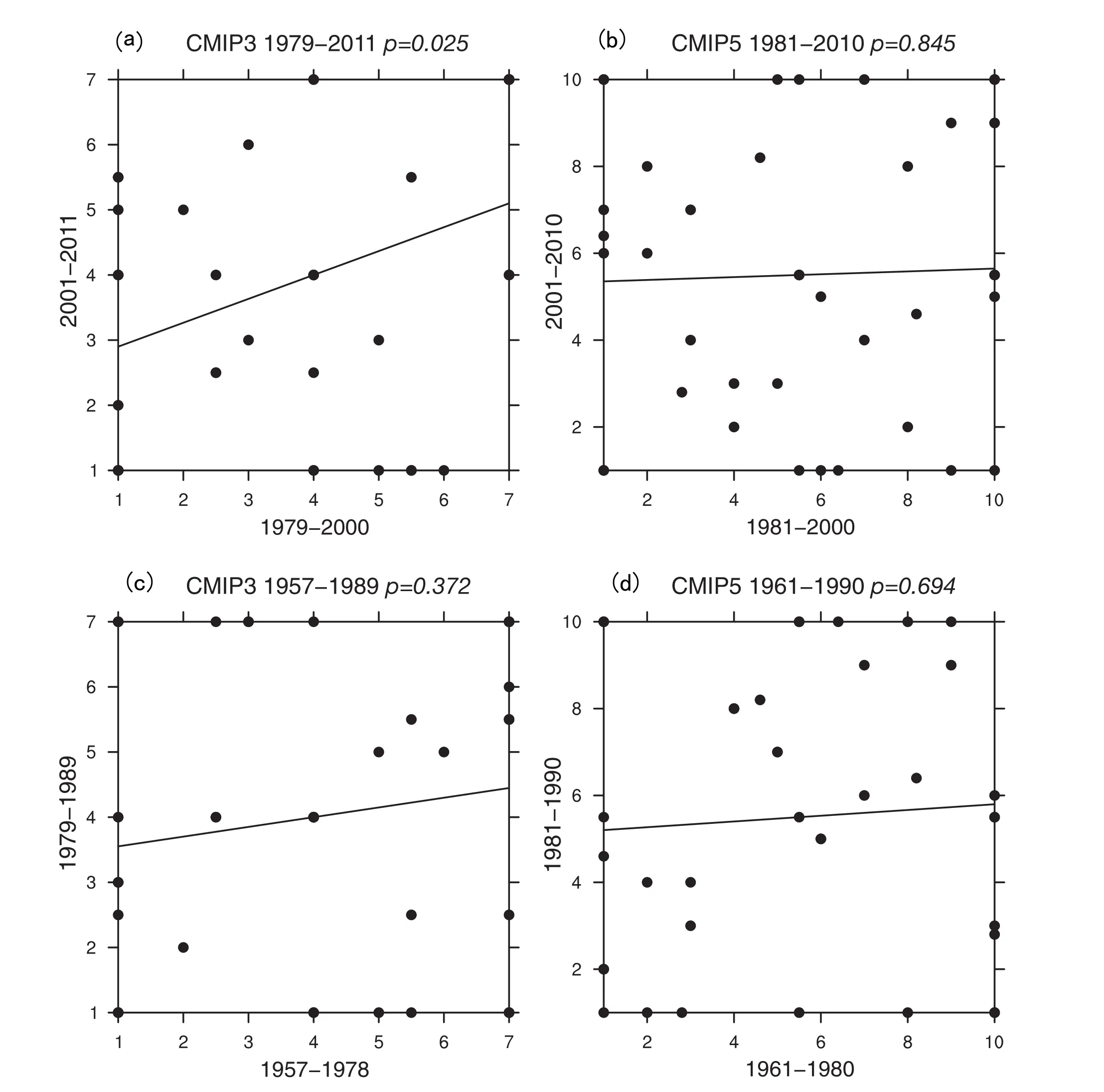
Fig.4.Regression between the ensemble ranks in DJF initialization and hindcast periods for(a)CMIP3 during 1979-2011,(b)CMIP5 during 1981-2010,(c)CMIP3 during 1957-1989,and(d)CMIP5 during 1961-1990.p values are based on reduced degrees of freedom from multiple GCMs,or samples.

Fig.5.SLP trends during DJF for 2001-2011 from(a)HadSLP2 observations,(b)the CMIP3 MME,(c)a subset of ensemble members from nine GCMs,(d)as(c)but all ensemble members from nine GCMs,(e)a subset of ensemble members from GISS-ER and GISS-EH,(f)as(e)but all ensemble members from GISS-ER and GISS-EH,(g)a subset of ensemble members from GFDL-CM2.1 and ECHAM5/MPI-OM,(h)as(g)but all ensemble members from GFDL-CM2.1 and ECHAM5/MPI-OM.

In addition to the spurious result that ranks are maintained in CMIP3 during 1979-2011,the average values and standard deviations do not change significantly in these hindcast experiments after excluding low performing ensemble members.Thus,ranking ensemble members by their past performance may not be a suitable method to improve the climate prediction skill.Similarly,selecting only one or a subset of ensemble members per model may underrepresent the actually simulated climate variability of that model.

Fig.6.As Fig.5,but for the 2001-2010 trends of CMIP5 historical multi-model mean and CMIP5 decadal ensemble members.

Different GCMs produce not only a different mean climate,but also a different variability between ensemble members.Fig.5 shows SLP trends for the 2001-2011 period.When comparing HadSLP2 observations(Fig.5a)to the CMIP3 multimodel mean trend(Fig.5b)that includes all available CMIP3 simulations(van Oldenborgh,2017),it becomes obvious that the trends in the multimodel mean are up to one order of magnitude lower than observed.Applying the exclusion process to the nine selected models described in Section 2(Fig.5c)suggests some minor improvement compared to including all ensemble members(Fig.5d),such as the positive trend around Greenland and the reduced erroneous positive trend over the Sargasso Sea in the North Atlantic,but the negative trend over western Europe and the positive trend over the Middle East are not as well represented.In general,the nine-model ensemble shows a similar spatial variability to the CMIP3 multimodel mean for large-scale trend detections.For the two models with large similarity between initialization and hindcast rankings,GISS-ER and GISS-EH,the spatial variability remains similar between all and all but excluded ensemble members(Fig.5e-f).However,it should be noted that these models were ranked low in a model comparison study with regard to their climate representation(Gleckler et al.,2008).On the other hand,the example of GFDL-CM2.1 and ECHAM5/MPI-OM(Fig.5g-h)shows a strong increase in spatial variability of decadal prediction after excluding poor performing ensemble members:the general strength of trends is improved and trends over many regions such as the west coast of the Americas,the Middle East,central Russia,and Australia appear closer to the observed.However,other regions such as western Europe remain in the wrong phase,making the interpretation of these trends dif ficult due to the large spatial inaccuracies in many regions.Also,trends in many subsets of the MME are largely non-significant.

Because individual ensemble members can have different probabilities for the likelihood that the trend is significant,we used Fisher's combined probability test(Mosteller and Fisher,1948)to identify the likelihood that the previously described SLP trends are statistically significant in an ensemble average:

Table 5As Table 3,but for the 10-year hindcast period 2001-2010.

withpibeing thep-values for trends of each ensemble memberi,withkbeing the number of ensemble members,and with χ22kbeing the χ2value for2k.

Predictions with decadal CMIP5 ensemble members(Fig.6)are compared to a MME that includes the seven CMIP5 models listed in Table 1(Fig.6c-d)and the MME of all available historical CMIP5 simulations(van Oldenborgh,2017)(Fig.6b).Compared to the CMIP3 multimodel mean SLP trends(Fig.5b),significant negative trends over South America and around southwest Africa and the strength of positive trends over the North and South Pacific are better represented in the CMIP5 MME,and positive trends over Greenland and negative trends over Europe and eastern Antarctica are less well simulated by the historical experiments during this decade.Despite the large differences in HadSLP2 observations when adding a single year(2011)to the trend calculations(Figs.5a and 6a)that indicate the strong year-to-year variability in seasonal SLP values,CMIP5 decadal predictions(Fig.6c-f)appear to simulate improved trend patterns compared to the multi-model mean.CanCM4 and FGOALS-g2 show similar trends to observations10See Table A3 in https://www.cs.umn.edu/sites/cs.umn.edu/ files/tech_reports/18-002.pdf.and FGOALS-g2 and CanESM2,which has a similar setup to CanCM4,simulate relatively realistic SAM patterns(Zheng et al.,2013).Boer et al.(2013)used CanCM4 to conclude that the effect of initialization diminishes beyond about a three-year average and the skill of the initialized forecast begins to approach that of the uninitialized simulation with both exhibiting modestly increasing skill with increasing averaging time.However,removing worse performing ensemble members does not affect the global SLP trend pattern in this subset of models(Fig.6e-f),which corroborates the hypothesis that the significant relationships between initialization and hindcast periods in the CMIP3 patterns are spurious.

Table 5 shows HadSLP2 trends and trend anomalies for the same ensemble members as in Table 3,but for the hindcast period.As in Fig.6,trend anomalies were taken with respect to the 2001-2010 hindcast period.The CMIP5 MMEs are less sensitive to the selection of appropriate ensemble members and the standard deviations in CMIP5 are generally higher than in CMIP3.Similar to Table 3,Table 5 does not indicate an improvement in the average simulated trend after excluding the worst performing CMIP5 ensemble members.It is suggested that this increase in variability is related to the representation of more processes in greater detail(Knutti and Sedlacek,2013).

4.Summary and conclusion

In this study,we describe a spurious pattern in decadal SLP trend predictions as simulated by a subset of CMIP3 models that is only present during the satellite era of 1979-2011.Wefind that such prejection skills are not present in CMIP3 model simulations during the earlier 1957-1989 period or in the more recent decadal CMIP5 predictions.This warrants caution when interpreting decadal prediction skill based on limited data.Consequently,it is also shown that results from a hindcast period of ensemble prediction experiments do not necessarily benefit from excluding ensemble members with poor performance during an initialization period.

The performance of individual ensemble members is described by ranking them based on their representation of global patterns in SLP.Previous studies have shown the importance of realistic SST initializations for decadal predictions (Keenlyside et al.,2008).For example,van Oldenborgh et al.(2012)found in a comparison of a fourmodel prediction with the CMIP3 MME that the decadal skill in the northern North Atlantic and eastern Pacific is most likely due to model initialization,whereas the skill in the subtropical North Atlantic and western North Pacific are likely due to the GHG and aerosol forcing.Yeager et al.(2012)suggested that the trend of ocean heat content between the subpolar and subtropical gyres in the North Atlantic is strongly in fluential on large-scale climate variability.

The method in the present paper first shows the variability of decadal SLP predictions and offers a comparison of different ensemble member simulations compared to the widely used method ofselecting only one(often thefirstavailable)ensemble member per model for model comparison.Secondly,we test if there is a relationship between SLP patterns in decadal model initializations and the following decade,or hindcast period.In the presented example,a statistically significant relationship is detected whereby half of the CMIP3 ensemble members retain their ranks based on a 22-year initialization or training period during a hindcast or testing period of 11 years.

Thirdly,we find that this relationship cannot be verified during the earlier 1957-1989 period,where 14 out of 38 ensemble members retain their ranks.Furthermore,these numbers are greatly reduced in decadal CMIP5 simulations,indicating an increase in spatial SLP variability in CMIP5 compared to CMIP3.Thus,despite the statistically significant relationship in the 1979-2011 CMIP3 simulations,the predictive value of the present approach cannot be corroborated during other periods or with CMIP5 models.

The reduced relationship for the 1957-1989 period is likely a result of the opposite AMO phase and lower trends during the initialization period,where the shift from positive to negative AMO phase in the early 1960's(Denton and Broecker,2008;Sutton and Hodson,2005)is counteracting the warming over high-latitude regions due to GHG emissions(Dima and Lohmann,2007;Hegerl et al.,1997).This results in reduced trends during the initialization period,and thus reduced skill during the hindcast period,when compared to the later 1979-2011 period.

In summary,this study highlights the importance of model intercomparison projects,not only between different GCMs,but also between different generations of models and different simulation time periods for model evaluation.Because of the significant in fluence of decadal climate variability on human well-being and our natural resources,it is important that predictions of future climate change accurately portray the plausible outcomes.

Acknowledgments

We would like to thank the two anonymous reviewers,whose insightful comments improved this manuscript.HadSLP2 data were received from the UK Met Of fice Hadley Centre Observations website.CMIP3 data were received from the PCMDI server and CMIP5 data were obtained from the Earth System Grid.Multi-modelmean valuesforboth CMIP3 and CMIP5 were retrieved from the KNMI Climate Explorer.The trend analysis was performed at the Minnesota Supercomputing Institute.

An earlier version of this manuscript benefited from the help of undergraduate researchers D.Ormsby and G.D.Smith at the University of Minnesota.Support for this study was provided by the U.S.National Science Foundation(1029711),the U.S.National Aeronautics and Space Administration(14-CMAC14-0010),and the George R.and Orpha Gibson Foundation at the University of Minnesota.

References

Allan,R.,Ansell,T.,2006.A new globally complete monthly historical gridded mean sea level pressure dataset(HadSLP2):1850-2004.J.Clim.19,5816-5842.

Arblaster,J.M.,Meehl,G.A.,2006.Contributions of external forcings to southern annular mode trends.J.Clim.19,2896-2905.

Bellucci,A.,Haarsma,R.,Bellouin,N.,etal.,2015.Advancementsin decadalclimate predictability:the role of nonoceanic drivers.Rev.Geophys.53,165-202.

Boer,G.J.,Kharin,V.V.,Merry field,W.J.,2013.Decadal predictability and forecast skill.Clim.Dyn.41,1817-1833.

Branstator,G.,2002.Circumglobal teleconnections,the jet stream waveguide,and the North Atlantic oscillation.J.Clim.15,1893-1910.

Casado,M.J.,Pastor,M.A.,2012.Use of variability modes to evaluate AR4 climate models over the Euro-Atlantic region.Clim.Dyn.38,225-237.

Chylek,P.,Li,J.,Dubey,M.,et al.,2011.Observed and model simulated 20th century arctic temperature variability:Canadian Earth system model CanESM2.Atmos.Chem.Phys.Discuss.11,22893-22907.

Collins,M.,2007.Ensembles and probabilities:a new era in the prediction of climate change.Phil.Trans.Roy.Soc.365A,1957-1970.

Collins,W.D.,Bitz,C.M.,Blackmon,M.L.,et al.,2006.The community climate system model version 3(CCSM3).J.Clim.19,2122-2143.

Delworth,T.L.,Broccoli,A.J.,Rosati,A.,et al.,2006.GFDL's CM2 global coupled climate models.part I:formulation and simulation characteristics.J.Clim.19,643-674.

Delworth,T.L.,Zhang,R.,Mann,M.E.,2007.Decadal to Centennial Variability of the Atlantic from Observations and Models,Ocean Circulation:Mechanisms and Impacts-Past and Future Changes of Meridional Overturning.AGU,Washington,DC.

Denton,G.H.,Broecker,W.S.,2008.Wobbly ocean conveyor circulation during the Holocene?Quat.Sci.Rev.27,1939-1950.

Dima,M.,Lohmann,G.,2007.A hemispheric mechanism for the Atlantic multidecadal oscillation.J.Clim.20,2706-2719.

Ding,Q.,Wang,B.,2005.Circumglobal teleconnection in the Northern Hemisphere summer.J.Clim.18,3483-3505.

Flatau,M.,Kim,Y.-J.,2013.Interaction between the MJO and polar circulations.J.Clim.26,3562-3574.

Gent,P.R.,Danabasoglu,G.,Donner,L.J.,et al.,2011.The community climate system model version 4.J.Clim.24,4973-4991.

Gerber,E.P.,Polvani,L.M.,Ancukiewicz,D.,2008.Annular mode time scales in the Intergovernmental Panel on Climate Change fourth assessment report models.Geophys.Res.Lett.35.L22707.

Gerber,E.P.,Baldwin,M.P.,Akiyoshi,H.,et al.,2010.Stratosphere-troposphere coupling and annular mode variability in chemistry-climate models.J.Geophys.Res.115.D00M06.

Gillett,N.P.,Fyfe,J.C.,2013.Annular mode changes in the CMIP5 simulations.Geophys.Res.Lett.40,1189-1193.

Gillett,N.P.,Stott,P.A.,2009.Attribution of anthropogenic in fluence on seasonal sea level pressure.Geophys.Res.Lett.36,.L23709.

Gillett,N.P.,Thompson,D.W.J.,2003.Simulation of recent Southern Hemisphere climate change.Science 302,273-275.

Gillett,N.P.,Zwiers,F.W.,Weaver,A.J.,et al.,2003.Detection of human in fluence on sea-level pressure.Nature 422,292-294.

Gillett,N.P.,Allan,R.J.,Ansell,T.J.,2005.Detection ofexternalin fluence on sea levelpressurewith amulti-modelensemble.Geophys.Res.Lett.32.L19714.

Gillett,N.P.,Fyfe,J.C.,Parker,D.E.,2013.Attribution of observed sea level pressure trends to greenhouse gas,aerosol,and ozone changes.Geophys.Res.Lett.40,2302-2306.

Gleckler,P.J.,Taylor,K.E.,Doutriaux,C.,2008.Performance metrics for climate models.J.Geophys.Res.113.D06104.

Handorf,D.,Dethloff,K.,2012.How well do state-of-the-art atmosphereocean general circulation models reproduce atmospheric teleconnection patterns?Tellus A Dyn.Meteorol.Oceanogr.64,19777.

Hegerl,G.C.,Hasselmann,K.,Cubasch,U.,et al.,1997.Multi- fingerprint detection and attribution analysis of greenhouse gas,greenhouse gas-plusaerosol and solar forced climate change.Clim.Dyn.13,613-634.

Hurrell,J.W.,1995.Decadal trends in the North Atlantic Oscillation:regional temperatures and precipitation.Science 269,676-679.

Hurrell,J.W.,1996.In fluence of variations in extratropical wintertime teleconnections on Northern Hemisphere temperature.Geophys.Res.Lett.23,665-668.

Karpechko,A.Y.,Gillett,N.P.,Marshall,G.J.,et al.,2009.Climate impacts of the southern annular mode simulated by the CMIP3 models.J.Clim.22,3751-3768.

Keenlyside,N.S.,Latif,M.,Jungclaus,J.,et al.,2008.Advancing decadalscale climate prediction in the North Atlantic sector.Nature 453,84-88.

Kim,H.-M.,Webster,P.J.,Curry,J.A.,2012.Evaluation of short-term climate change prediction in multi-model CMIP5 decadal hindcasts.Geophys.Res.Lett.39.L10701.

Knutti,R.,Sedlacek,J.,2013.Robustness and uncertainties in the new CMIP5 climate model projections.Nat.Clim.Change 3,369-373.

Laepple,T.,Jewson,S.,Coughlin,K.,2008.Interannual temperature predictions using the CMIP3 multi-model ensemble mean.Geophys.Res.Lett.35.L10701.

Latif,M.,Arpe,K.,Roeckner,E.,2000.Oceanic controlofdecadalNorth Atlantic sea level pressure variability in winter.Geophys.Res.Lett.27,727-730.

Lee,M.-Y.,Hsu,H.-H.,2013.Identification of the Eurasian-North Pacific multidecadal oscillation and its relationship to the AMO.J.Clim.26,8139-8153.

Li,L.,Lin,P.,Yu,Y.,et al.,2013.The flexible global ocean-atmosphere-land system model,Grid-point Version 2:FGOALS-g2.Adv.Atmos.Sci.30,543-560.

Liess,S.,Kumar,A.,Snyder,P.K.,et al.,2014.Different modes of variability over the Tasman Sea:implications for regional climate.J.Clim.27,8466-8486.

Liess,S.,Agrawal,S.,Chatterjee,S.,et al.,2017.A teleconnection between the West Siberian Plain and the ENSO region.J.Clim.30,301-315.

L'Heureux,M.L.,Thompson,D.W.J.,2006.Observed relationships between the El Ni~no-southern oscillation and the extratropical zonal-mean circulation.J.Clim.19,276-287.

Mahajan,S.,Zhang,R.,Delworth,T.L.,2011a.Impact of the Atlantic Meridional Overturning Circulation(AMOC)on Arctic surface air temperature and sea ice variability.J.Clim.24,6573-6581.

Mahajan,S.,Zhang,R.,Delworth,T.L.,et al.,2011b.Predicting Atlantic Meridional Overturning Circulation(AMOC)variations using subsurface and surface fingerprints.Deep Sea Res.Part II Top Stud.Oceanogr.58,1895-1903.

Matei,D.,Baehr,J.,Jungclaus,J.H.,et al.,2012.Multiyear prediction of monthly mean atlantic meridional overturning circulation at 26.5°N.Science 335,76-79.

McFarlane,N.,Scinocca,J.,Lazare,M.,et al.,2005.The CCCma third generation atmospheric general circulation model.CCCma Internal Rep.25,16.

Medhaug,I.,Furevik,T.,2011.North Atlantic 20th century multidecadal variability in coupled climate models:sea surface temperature and ocean overturning circulation.Ocean Sci.7,389-404.

Meehl,G.A.,Goddard,L.,Murphy,J.,et al.,2009.Decadal prediction:can it be skillful?Bull.Am.Meteorol.Soc.90,1467-1485.

Miller,R.L.,Schmidt,G.A.,Shindell,D.T.,2006.Forced annular variations in the 20th century Intergovernmental Panel on Climate Change fourth assessment report models.J.Geophys.Res.111.D18101.

Mosteller,F.,Fisher,R.A.,1948.Questions and answers:combining independent tests of significance.Am.Statistician 2,30-31.

NASA,1976.US Standard Atmosphere.National Aeronautics and Space Administration,vol.243.United States Air Force,Washington,DC.

Nakicenovic,N.,Alcamo,J.,Davis,G.,de Vries,B.,Fenhann,J.,Gaf fin,S.,Gregory,K.,Grubler,A.,Jung,T.Y.,Kram,T.,2000.Emissions scenarios:summary for policymakers.In:Nakicenovic,N.,Swart,R.(Eds.),Special Report on Emissions Scenarios:A Special Report of Working Group III of the Intergovernmental Panel on Climate Change.Intergovernmental Panel on Climate Change Cambridge University Press,Cambridge and New York.

Nozawa,T.,Nagashima,T.,Tomo’o Ogura,T.Y.,et al.,2007.Climate Change Simulations with a Coupled Ocean-atmosphere GCM Called the Model for Interdisciplinary Research on Climate:MIROC,CGER Supercomput.Monogr,12 ed.Cent.For Global Environ.Res.,Natl.Inst.for Environ.Stud.,Tsukuba,Japan.

Pastor,M.A.,Casado,M.J.,2012.Use of circulation types classifications to evaluate AR4 climate models over the Euro-Atlantic region.Clim.Dyn.39,2059-2077.

Pincus,R.,Batstone,C.P.,Hofmann,R.J.P.,et al.,2008.Evaluating the present-day simulation of clouds,precipitation,and radiation in climate models.J.Geophys.Res.113.D14209.

Pohlmann,H.,Jungclaus,J.H.,K¨ohl,A.,et al.,2009.Initializing decadal climate predictions with the GECCO oceanic synthesis:effects on the North Atlantic.J.Clim.22,3926-3938.

Raddatz,T.,Reick,C.,Knorr,W.,et al.,2007.Will the tropical land biosphere dominate the climate-carbon cycle feedback during the twenty- first century?Clim.Dyn.29,565-574.

Roeckner,E.,Baeuml,G.,Bonaventura,L.,et al.,2003.The Atmospheric General Circulation Model ECHAM5 Part I:Model Description,Maxplanck-institut Fuer Meteorologie,349 ed.Max-Planck-Institut fuer Meteorologie,Hamburg,Germany.

Ruiz-Barradas,A.,Nigam,S.,Kavvada,A.,2013.The Atlantic Multidecadal oscillation in twentieth century climate simulations:uneven progress from CMIP3 to CMIP5.Clim.Dyn.41,3301-3315.

Sakamoto,T.,Komuro,Y.,Ishii,M.,et al.,2012.MIROC4h:a new highresolution atmosphere-ocean coupled general circulation model.J.Meteorol.Soc.Jpn.90,325-359.

Santer,B.D.,Wigley,T.M.L.,Boyle,J.S.,et al.,2000.Statistical significance of trends and trend differences in layer-average atmospheric temperature time series.J.Geophys.Res.105,7337-7356.

Schmidt,G.A.,Ruedy,R.,Hansen,J.E.,et al.,2006.Present-day atmospheric simulations using GISS ModelE:comparison to in situ,satellite,and reanalysis data.J.Clim.19,153-192.

Schubert,S.,Wang,H.,Suarez,M.,2011.Warm season subseasonal variability and climate extremes in the Northern Hemisphere:the role of stationary Rossby waves.J.Clim.24,4773-4792.

Simmonds,I.,2015.Comparing and contrasting the behaviour of Arctic and Antarctic sea ice over the 35 year period 1979-2013.Ann.Glaciol.56,18-28.

Stoner,A.M.K.,Hayhoe,K.,Wuebbles,D.J.,2009.Assessing general circulation model simulations of atmospheric teleconnection patterns.J.Clim.22,4348-4372.

Sutton,R.T.,Hodson,D.L.R.,2005.Atlantic ocean forcing of North American and European summer climate.Science 309,115-118.

Teng,H.,Branstator,G.,Wang,H.,et al.,2013.Probability of US heat waves affected by a subseasonal planetary wave pattern.Nat.Geosci.6,1056-1061.

Trenberth,K.E.,1981.Seasonal variations in global sea level pressure and the total mass of the atmosphere.J.Geophys.Res.86,5238-5246.

Trenberth,K.E.,1991.Storm tracks in the southern hemisphere.J.Atmos.Sci.48,2159-2178.

Trenberth,K.E.,Stepaniak,D.P.,Smith,L.,2005.Interannual variability of patterns of atmospheric mass distribution.J.Clim.18,2812-2825.

van Oldenborgh,G.J.,2017.KNMI Climate Explorer.https://climexp.knmi.nl.

van Oldenborgh,G.J.,Doblas-Reyes,F.,Wouters,B.,et al.,2012.Decadal prediction skill in a multi-model ensemble.Clim.Dyn.38,1263-1280.

van Vuuren,D.P.,Edmonds,J.,Kainuma,M.,et al.,2011.The representative concentration pathways:an overview.Clim.Change 109,5-31.

Walsh,J.E.,Chapman,W.L.,Shy,T.L.,1996.Recent decrease of sea level pressure in the central Arctic.J.Clim.9,480-486.

Watanabe,M.,Suzuki,T.,O’ishi,R.,et al.,2010.Improved climate simulation by MIROC5:meanstates,variability,andclimatesensitivity.J.Clim.23,6312-6335.

Wilmes,S.B.,Raible,C.C.,Stocker,T.F.,2012.Climate variability of the midand high-latitudes of the Southern Hemisphere in ensemble simulations from 1500 to 2000 AD.Clim.Past 8,373-390.

Xin,X.-G.,Zhou,T.-J.,Yu,R.-C.,2008.The Arctic Oscillation in coupled climate models.Chin.J.Geophys.51,223-239.

Yeager,S.,Karspeck,A.,Danabasoglu,G.,et al.,2012.A decadal prediction case study:late twentieth-century North Atlantic Ocean heat content.J.Clim.25,5173-5189.

Yu,Y.,Zheng,W.,Wang,B.,et al.,2011.Versions g1.0 and g1.1 of the LASG/IAP flexible global ocean-atmosphere-land system model.Adv.Atmos.Sci.28,99-117.

Yukimoto,S.,Noda,A.,Kitoh,A.,et al.,2006.Present-day climate and climate sensitivity in the meteorological research Institute coupled GCM version 2.3(MRI-CGCM2.3).J.Meteorol.Jpn.Ser.II 84,333-363.

Yukimoto,S.,Adachi,Y.,Hosaka,M.,et al.,2012.A new global climate model of the Meteorological Research Institute MRI-CGCM3-Model description and basic performance.J.Meteorol.Soc.Jpn.90A,23-64.

Zhang,L.,Wang,C.,2013.Multidecadal North Atlantic sea surface temperature and Atlantic meridional overturning circulation variability in CMIP5 historical simulations.J.Geophys.Res.118,5772-5791.

Zheng,F.,Li,J.,Clark,R.T.,et al.,2013.Simulation and projection of the Southern Hemisphere annular mode in CMIP5 models.J.Clim.26,9860-9879.