
Fixed-time Consensus for Leader-follower Second-order Multi-agent Systems
2019-10-30 10:18CHENMaoliWANGXiao
CHEN Mao-li, WANG Xiao
(College of Liberal Arts and Sciences, National University of Defense Technology, Changsha, 410073,P.R. China)
Abstract:We analyse the fixed-time consensus problem for multi-agent systems with leaderfollower mode. Based on a follower’s observation structure for the leader’s information, it is proved that the estimation errors can be converged to zero at a fixed time. From this stability and a sliding mode structure, we derive a control input of followers, which provides a critical support for fixed-time consensus. The simulation results demonstrate that this control approach does conduce to the implementation of the fixed-time synchronization.
Key words: Leader-follower synchronization; Fixed-time stability; Multi-agent Systems
§1. Introduction
In recent decades, the research on the synchronization control problem of multi-agent systems has never been attenuated, and it has been widely used in the fields of unmanned control,social sciences, physics and others [1-2]. Inspired by the theoretical framework for the establishment of first-order multi-agent system consensus problems by Olfati-Saber and Murray in[4], some scholars have proposed a number of novel multi-agent control protocols [6, 12-13].However, most of the research results of scientists and engineers in control engineering have focused on Lyapunov asymptotic stability (i.e. infinite time intervals). In practical applications,one of the main concerns is on the property of trajectory to the system over a finite or fixed interval. It is because of what there are several examples where the state variable is too large to be applied. To solve these problems, Dorato first introduced the concept of finite time stability in 1961 in[10]. The finite time stability means that the system state reaches the expected value for a limited period of time, which is not possible with asymptotic stability and which also satisfies the needs of the application system.
As yet, most of the results have been processed the system to achieve synchronization in a finite time. However, as an extension of finite time stability, there’s been very little work done on the fixed-time consistency or synchronization in the study of multi-agent system control.Fixed-time stability problem was first proposed in[11]and presented in[7], that is, the settling time of the system is uniformly bounded and has nothing to do with the initial conditions. In[7],a precise estimation bound for the stability time is given for a first-order system. Furthermore,the fixed-time consensus design framework of the first-order system is generalized in[8]. For the control problem of higher-order systems, in the recent work of [15], the authors give an upper bound of the stability time, which does not depend on the initial conditions. Although limited reports on the fixed-time stability of multi-agent systems are available, such as [16] and [17],some results have been published and affirmed by many scholars. Therefore, it is significant and imperative to further explore the fixed time stability of multi-agent systems.
In this work, we consider a system with N+1 agents, including one leader labeled by 0 and N followers labeled by i=1,2,··· ,N. The dynamics model of the leader are depicted by

where x0(t), v0(t), u0(t) ∈R represents the position, velocity and a predetermined input of the leader. The dynamics model of the ith follower are governed by

Here xi(t), vi(t), ui(t) ∈R represents the position, velocity and a control input of the ith follower. ∆i(t) represents the uncertain disturbance. One of the purposes of this paper is to obtain an appropriate ui(t) such that System (1.1)-(1.2) achieve consensus at a fixed time.
Remark 1.1System (1.1)-(1.2) is described from the perspective of graph theory. The connection among the followers can be characterized by a digraph G = {V,ε}, where V ={1,2,··· ,N}, ε = V ×V. The adjacency matrix is denoted by A = (aij)N×N. If there is a direct connection between the follower i and j,then aij=1. Otherwise,aij=0. The connection between the leader and the follower is described by a diagonal matrix B = diag{b1,··· ,bN}.Ifit means that the ith follower can connect directly with the leader.
Assumption 1.1
(1) Graph G is connected and, i.e. there is i ∈{1,2,··· ,N} such that
(2) The interference terms of all the followers in the system are uniformly bounded, that is,there exists δ >0 such that |∆i(t)|≤δ for all i ∈{1,2,··· ,N}.
The structure of this paper is designed as follows. Some definitions and classic auxiliary lemmas are reviewed and briefly stated in Section 2. Based on Lyapunov method and a sliding mode structure,the fixed-time consensus conditions of System(1.1)-(1.2)and its stability analysis are accomplished in Section 3. Numerical simulations are listed in Section 4 to illustrate the validity of theoretical results. Section 5 is dedicated to summarizing this work and stating concisely future discussions.
§2. Preliminaries
In this section, we recall the definition of fixed-time stability and the associated auxiliary lemmas. We still follow the definition of fixed-time stability proposed in [7].

Definition 2.1[7]Consider the following first-order system:where x ∈Rdand f :R+×Rd→Rdis a nonlinear function that satisfies f(0,0)=0. The origin of the following first-order system is said to be fixed-time stable if it is globally asymptotically stable,any solution x(t)of(2.1)reaches the equilibria at a settling time T,which is independent of initial conditions.
Lemma 2.1[7]If there exists a continuous radially unbounded and positive definite function V(x) such that

for some α, β, p, q, k > 0 and 0 < pk < 1, qk > 1, then the origin of this system (2.1) is globally fixed-time stable. The settling time function T can be estimated by

Furthermore, if p = 1+1/µ and q = 1 −1/µ with µ > 1 are selected, the settling time function T can be estimated by a less conservative bound

Lemma 2.2[7]Consider the system

where x=(x1,x2)T∈R2is the state vector and u(t)∈R is the control input. Let the positive constants ci>0(i=1,2) be such that both the polynomial y2+c2y+c1and y2+3c2y+3c1are Hurwitz in terms of the Laplace operator y. There exists a constant∈(0,1) such that,for every∈(0,1), the system (2.5) can be stabilized at the origin in a fixed-time under the control

with ϑi,=1,2) are determined by

The proof of Lemma 2.2 could be derived by following the same line as the proof of Theorem 2 given in [9].
§3. A Fixed-time Consensus Theorem
To accomplish a fixed-time leader-follower consensus of System (1.1)-(1.2), a control structure is selected to characterize the follower’s estimation of the leader’s information, inspired by the work of [5]. The fixed time convergence of these estimated values is of vital necessity in the acquisition of synchronization.
Let x0,i(t), v0,i(t) be the ith follower’s tracking estimates for the position and velocity of the leader and satisfy the following observation estimation structure:
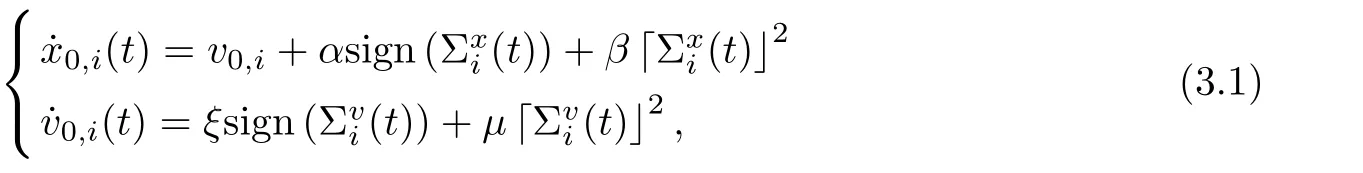


where1Nis the n-dimensional column vectors with all components of 1, and ⊗is the tensor product.
Below we point out that each follower can accurately estimate the status of the leader in a fixed interval, i.e., the error vectors xe, veconverge to zero at a fixed time.
Lemma 3.1If Assumption 1.1 hold. The observation coefficients ξ > 0, µ > 0, and ξ satisfy ξ >umax0 . Then the estimation error xe, veconverge to zero at a fixed time Tf, that is

ProofThe proof of the theorem is accomplished in the following two steps.
Step OneWe show that estimation errors are bounded at any [0,t], that is, xe,vedo not tend to infinity in a finite interval. Consider

Differentiate Q(t) along (3.3) and one obtained

where 2aTb ≤aTa+bTb andare used. Hence, Q(t) is bounded at any[0,t]. Further, xe, veare bounded at any finite time interval by (3.5).
Step TwoConsider the Lyapunov function

The derivative along the trajectory of the system (3.3) is

Therefore, by Lemma 2.1, veis stable at the origin at a fixed time, and an upper bound of time is

that means ve(t)=0,After the convergence of ve, the first equation of the system(3.3) reduce to

Similarly, xeis stable at the origin at a fixed time, and an upper bound of time is

Thus,

Remark 3.1 Lemma 3.1 shows that x0,i(t) = x0(t), v0,i(t) = v0(t) for all t ≥Tf.Moreover, it implies that the expected time Tfcan be obtained by setting the appropriate observation coefficients according to (3.4).
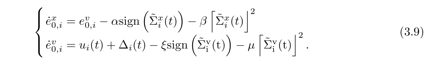
We next demonstrate the fixed-time consensus for(1.1)-(1.2). Letbe the difference between the true deviations and the estimated deviations of the position and velocity, that is,

By (3.2), the derivative ofwith respect to t is
Consider the following sliding mode surface for each follower:

where ci, ϑi, ϑ'i(i = 1,2) are the appropriate parameters selected in Lemma 2.2. Taking the second equation of (3.9), the derivative of si(t) along the solution of (3.9) is


where U(t)=(u1(t),··· ,uN(t))T, ∆(t)=(∆1(t),··· ,∆N(t))T. Moreover,(3.11)is reduced to

Therefore, consider
where ν >1, ς ≥δ and |∆i(t)|≤δ, i=1,2,··· ,N.
Theorem 3.1Fixed-time Consensus Theorem. Assume that the system (1.1)-(1.2)satisfies Assumption 1.1, the fixed-time leader-follower consensus can be achieved by (3.14).
ProofThe proof of the theorem is accomplished in the following three steps.
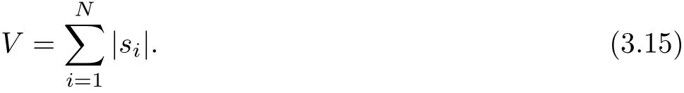
Step One)(i=1,2,··· ,N)are bounded at any[0,t],that is,(t)do not tend to infinity in a finite interval. Consider the Lyapunov function
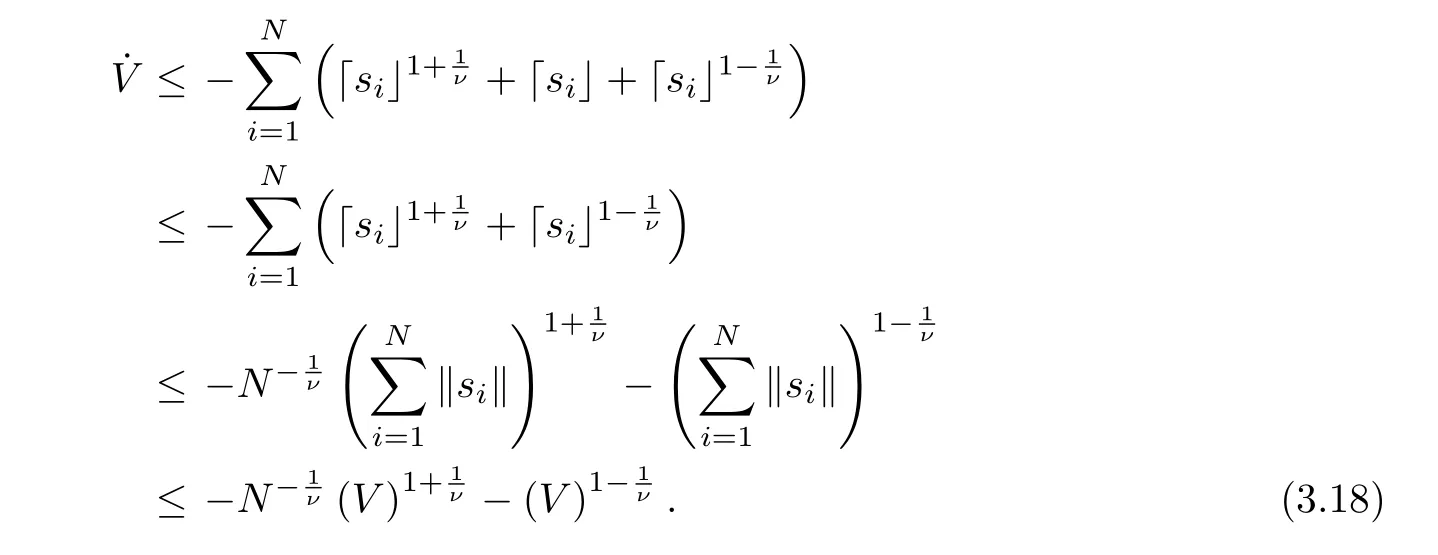
Thus, combining (3.11) with (3.14), the time derivative of V can be indicated by
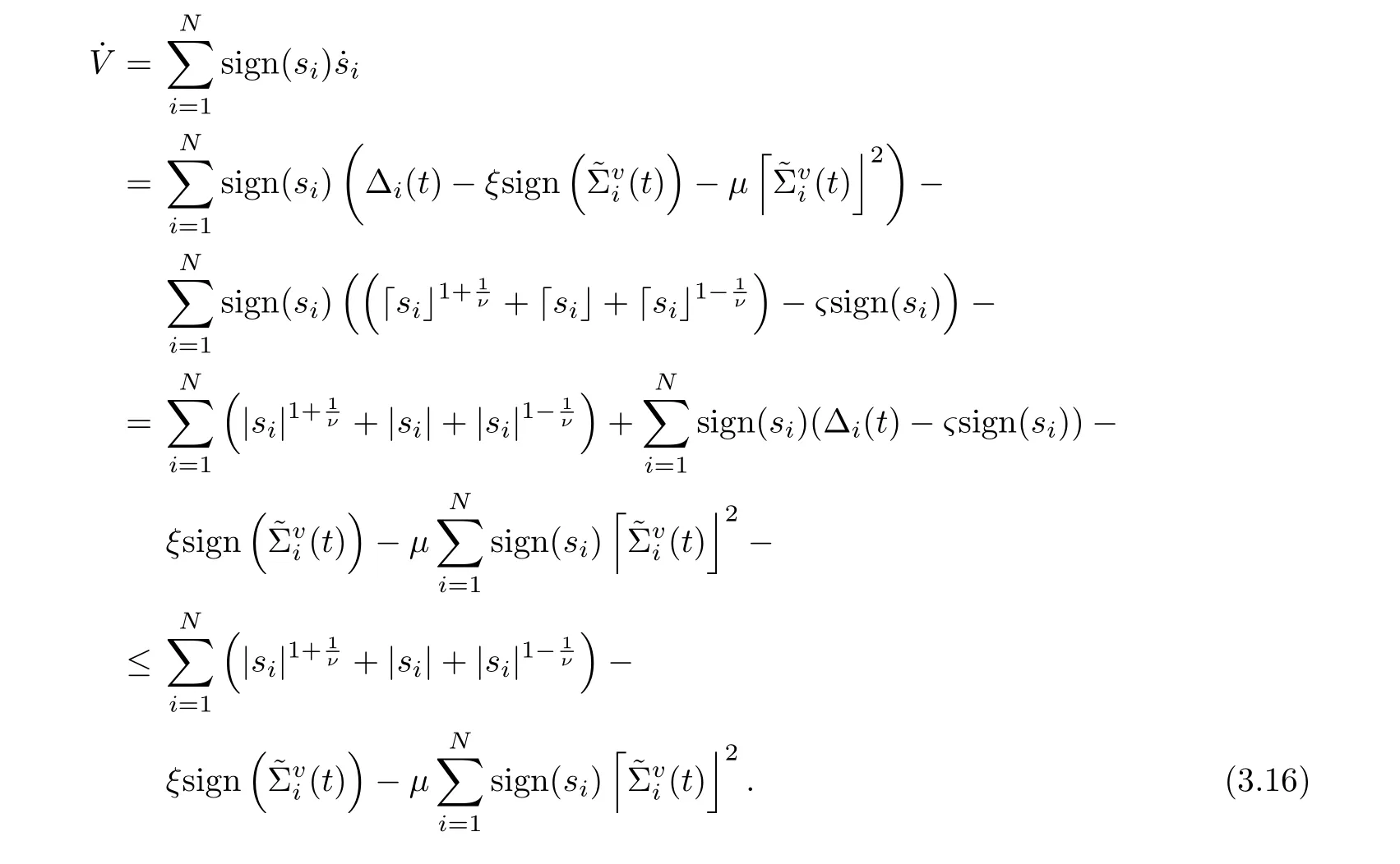
Here,the inequality is generated by Assumption 1.1 and ς ≥δ. By Lemma 2.3,converge to the origin at fixed time Tffor all i ∈{1,2,··· ,N}. It means thatare uniformly bounded at any [0,t], i.e.≤γ,≤γ for some γ > 0. Thus,there exists a constant C such that

It is straightforward to show that V is bounded at any[0,t]. Therefore,|si|(i=1,2,··· ,N)is bounded at any [0,t]. From (3.10), it can be known that)(i = 1,2,··· ,N) is bounded at any [0,t] by the boundedness of
Step TwoUnder the input control (3.14), it will reach the sliding surface si= 0 at a fixed time T1.
For ∀t ≥Tf, then (3.16) is reduced to
Following the Lemma 2.2, si(t)=0 for all t ≥Tf+T1with T1=
Step ThreeOn the sliding surface si=0,after the fixed time i.e. ex→0, ev→0.
For any t ≥Tf+T1, the err or system (3.12) is rewritten as

where Ex(t)=(Ex1(t),··· ,ExN(t))T,Ev(t)=(Ev1(t),··· ,EvN(t))Tand Exi(t), Evi(t)are defined in (3.10). By Lemma 2.2, there is a constant T2> 0, such that ex0,i(t) →0, ev0,i(t) →0 for t ≥Tf+T1+T2. This indicates that xi−x0→0, vi−v0→0, i=1,2,··· ,N.
§4. Numerical Simulations
In this section, simulation examples are provided to illustrate the validity of the theoretical results. A multi-agent system consists of one leader and four followers and the dynamic descriptions of leaders and followers are:

and

where xi(t), vi(t)∈R represent the position and velocity of ith follower. ui(t)∈R is the input item. ∆i(t) represents the uncertain disturbance.
For simplicity,we give the following assumptions to the leader: fixed position and no control inputs. Without loss of generality, let (x0,v0)T= (0,0)T. The parameters in the simulations are as follows: (i) c1= 2, c2= 3,0.5,0.8 in (2.6), it follows that ϑ1= 2/3,−1, ϑ2= 0.8,= −1.2 from (2.7); (ii) α = 0.8, β = 1.2, ξ = 2.0, µ = 1.2 in (2.1). The initial configuration of the followers are considered:
• Case1: (x1,v1)=(4,−20),(x2,v2)=(2,−10),(x3,v3)=(−2,10),(x4,v4)=(−4,20);
• Case2: (x1,v1)=(1.8,−9),(x2,v2)=(0.5,−3.5),(x3,v3)=(−0.3,2),(x4,v4)=(−1.5,5).
The simulation results are depicted intuitively in Figure 1 and Figure 2. As can be seen from these figures, the position and velocity deviation between each follower and leader decreases sharply and converges to zero. Although each follower converges at different times,their states are ultimately the same as the leader. This means that leader and followers can achieve synchronization within a certain amount of time.

Figure 1: Case1 (a): Positional deviation between each follower and leader;(b): Velocity deviation between each follower and leader.

Figure 2: Case2 (a): Positional deviation between each follower and leader;(b): Velocity deviation between each follower and leader.
§5. Conclusions
The fixed-time leader-follower consensus problem of multi-agent system is studied. Under certain assumptions, based on the Lyapunov method and a sliding mode control structure, the follower control input is obtained, which states an available method to achieve a fixed-time leader-follower consensus. The enumeration of two numerical simulations confirms the validity of the theoretical results. In practical applications, we pay more attention to the following two facts. For one thing, flocking behavior emerges in multi-agent systems. Specifically, the velocity of the system is synchronized and the relative positions between any two agents are bounded. For another, the existence of time delays caused by limited communication between agents. Since multi-agent systems are often affected by factors such as information transmission velocity and transmission congestion, delay is inevitable. Hence, we will consider the above two aspects. The one is the realization of leader-centered flocking, the other is committed to introducing delays into this research and considering the impact of time delays.
 Chinese Quarterly Journal of Mathematics2019年3期
- Chinese Quarterly Journal of Mathematics的其它文章
- Normality Criteria of Zero-free Meromorphic Functions
- On Uniqueness Problem of Meromorphic Functions Sharing Values with Their q-shifts
- Algorithm on the Optimal Vertex-Distinguishing Total Coloring of mC9
- Finite Difference Methods for the Time Fractional Advection-diffusion Equation
- Globally Bounded Solutions in A Chemotaxis Model of Quasilinear Parabolic Type
- Triple Positive Solutions for a Third-order Three-point Boundary Value Problem