Damage identification of steel truss bridges based on deep belief network

Tu Yongming Lu Senlu Wang Chao

(Key Laboratory of Concrete and Prestressed Concrete Structures of Ministry of Education,Southeast University, Nanjing 211189, China)(National Prestressing Engineering Research Center, Southeast University, Nanjing 211189, China)(School of Civil Engineering, Southeast University, Nanjing 211189, China)

Abstract：To improve the accuracy and anti-noise ability of the structural damage identification method, a bridge damage identification method is proposed based on a deep belief network (DBN). The output vector is used to establish the nonlinear mapping relationship between the mode shape and structural damage. The hidden layer of the DBN is trained through a layer-by-layer pre-training. Finally, the backpropagation algorithm is used to fine-tune the entire network. The method is validated using a numerical model of a steel truss bridge. The results show that under the influence of noise and modeling uncertainty, the damage identification method based on the DBN can identify the accurate damage location and degree identification compared with the traditional damage identification method based on an artificial neural network.

Key words：deep learning; restricted Boltzmann machine; deep belief network; structural damage identification

Civil engineering is closely related to people’s life and property during construction and service. The collapse of high-rise buildings and long-span bridges will cause devastating damage. Hence, it is of great significance to ensure the safety of civil engineering structures during construction and service. However, due to the aging of materials, initial design defects, unqualified quality during construction, and the influence of earthquakes, wind loads, traffics, temperatures, corrosions, and other environmental factors during usage, various types of damage can easily occur during the construction and use of structures. The damage to structures often occurs with the degradation of their physical properties, such as cross-section cracking and mass reduction, which affects their dynamic characteristics, such as frequency and stiffness. Hence, how to find the location and degree of the damage to such structures in time is of great significance. Based on the vibration characteristics of structures, several structural damage identification methods have been developed. Such methods are based on the fact that structural cross-section and mass changes influence the vibration characteristics of the structure and allow a rapid and global assessment of large structures. However, the difficulty for vibration testing is that noise, uncertainty in modeling, and the sensitivity of selected indicators to damage may adversely affect the damage identification results. In recent years, the use of artificial intelligence methods for structural damage identification has become a hotspot. From the perspective of mathematical methods, structural damage identification is essentially a pattern recognition problem. Machine learning is a good tool for pattern recognition. Santos et al.[1]used a Gaussian mixture model (GMM) based on a genetic algorithm and expectation maximization (EM) algorithm to evaluate the damage of the Z24 bridge through the change in frequency. The research shows that the GA-EM-GMM can distinguish that the change in frequency is caused by the damage and temperature. An autoregressive (AR) model[2]was established to describe the acceleration time series. Principal component analysis (PCA) and Sammon mapping were used to reduce the dimension of the AR coefficient matrix. Then, learning vector quantization and nearest neighbor classification algorithm were used to monitor and classify the damage condition of a laboratory simple three-layer framework and ASCE standard structure. The research shows that this method can effectively evaluate the damage condition. The damage status of the structure was analyzed, and different damage degrees were classified. Gui et al.[3]used a support vector machine (SVM) based on an optimization algorithm to identify the damage to a three-layer aluminum frame in a laboratory. The research shows that a residual error is more sensitive to damage signals than the AR parameter and can judge the damage state of structures more accurately. Therefore, selecting the appropriate damage feature in the SVM for damage classification is very important. Ozdagli et al.[4]validated a simply supported beam numerical model, a laboratory 2D three-layer measured frame model, and a laboratory 3D frame model using PCA and a self-encoder (AE). Through the data reconstruction of input data, the Euler distance constructed by the residual error of the input and output was used to evaluate the variability of the structural model and structural health condition. The research shows that the modal shape is more sensitive to damage than the frequency and is not affected by the temperature. However, the frequency alone is not sensitive to the small damage and is greatly affected by the temperature, so judging whether the variability of the results is caused by the damage or temperature is impossible. Bandara et al.[5]formulated a new damage index by reducing the dimension of the frequency response function matrix by PCA and then established the relationship between the damage index and damage degree using artificial neural networks (ANNs). The research shows that ANNs can identify the damage condition of a structure, but they divide a two-story frame structure into 14 parts and establish 14 ANNs, which is of great significance to large-scale geotechnical engineering. Lam et al.[6]proposed to use Bayesian design ANNs to detect the location and severity of the damage based on the change in the Ritz vector caused by the damage. Successful identifications and applications have been achieved using the above-mentioned methods. Among the ANN methods, the gradient descent algorithm is one of the most commonly used algorithms for training neural networks. However, when using these algorithms to train samples, especially in the case of several hidden layers in a network, the gradient disappearance problem may occur. Furthermore, the machine learning method has high requirements on the damage index, so it is often necessary to construct a damage index that is more sensitive to damages. Secondly, for large bridges or high structures, the combination of damage location and damage degree is amazing. However, machine learning algorithms, such as SVMs and ANNs, cannot easily locate and quantify damages because of their shallow structure, which is often used to study a specific damage condition or just health. In recent years, deep learning algorithms have become a research hotspot because of their strong nonlinear analysis ability and the ability to extract high-dimensional features. Their requirements for the damage index are not high. They often need only the frequency, vibration mode, or acceleration data to establish a relationship with the damage status and then accurately realize the identification of the damage location and damage degree. Nadith et al.[7]used an autoencoder model with a deep neural network structure to perform a numerical simulation and experimental verification on a steel frame structure through layered pre-training and fine-tuning. The results show that, compared with traditional ANNs, this method can identify the location and degree of damage and improve accuracy and efficiency. Zhang et al.[8]used a one-dimensional convolutional neural network to input the original acceleration data into the convolutional neural network. The research shows that a one-dimensional convolutional neural network is more sensitive to the small local damage of a structure, can effectively extract the high-dimensional features of the damage, and has a strong anti-noise performance. Guo et al.[9]used a deep belief network (DBN) to identify the damage to a real bridge. The research shows that the DBN is more accurate than a backpropagation (BP) neural network in identifying the damage to a bridge, but it specifies several specific locations in the identification of the damage location. The identification of the damage location in these specific locations has certain limitations.

The above research shows that a deep learning algorithm can effectively extract high-dimensional damage features, and the requirement of the damage index is not high.

In this study, the DBN is used for structural damage identification. The model can extract the high-dimensional features of damage to establish the nonlinear mapping relationship between vibration characteristics and damage. A numerical model of a steel truss bridge in Sweden was established to obtain modal characteristics, such as modal shape. The modal shape of the structure was taken as the input vector of the training model, and its damage was taken as the output vector of the training model. The training process was divided into two parts: A part of the training set was used for pre-training to determine a group of good weights and thresholds. The remaining training set was fine-tuned to obtain the optimal weight and threshold. The accuracy and efficiency of the method were verified using a numerical example of the steel truss bridge.

1 Structural Health Monitoring Framework Based on a DBN

1.1 Restricted Boltzmann machine

The restricted Boltzmann machine (RBM) is the basic model of DBNs, and it is an undirected graph model of the dictograph structure. The variables in the RBM are also divided into implicit and observable variables, as shown in Fig.1. The observable layer and hidden layer can be used to represent the two groups of variables, respectively. There is no connection between nodes in the same layer. All nodes of the layer are connected, which is the same as the structure of a two-layer fully connected neural network.

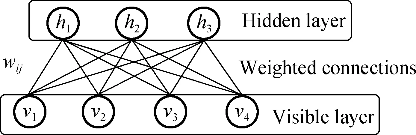
Fig.1 RBM

An RBM consists ofKvobservable variables andKhhidden variables, whose definition is as follows:

1) Observable random vectorsv∈RKv.

2) Hidden random vectorsh∈Rkh.

3) Weight matrixw∈Rkv×kh. Each elementwijis the weight between the observable variableviand hidden variablehj.

4) Biasa∈RKvandb∈Rkh, whereaiis the bias of each observable variableviandbjis the bias of each hidden variablehj.

The RBM is an energy-based model; that is, the combination state of each model variable corresponds to an energy, and the training process of the model is the process of constantly changing energy. In the state of the known visible layer and hidden layer neuron, the energy function is defined as

(1)

The joint probability distribution of the RBM is defined as

(2)

Because there is no connection between the variables in the same layer of the RBM, the hidden variables are independent of one another when the observable variables are given. Similarly, when the hidden variables are given, the observable variables are also conditionally independent of one another. Based on the above conditions, it can be deduced that the RBM is a network model whose activation function isf(x)=sigmoid(x), and the conditional probabilities of each observable variable and hidden variable are

(3)

(4)

whereσis the logistic function.

The RBM uses the maximum likelihood function to determine the optimal parameters. Given a group of training samples, the log likelihood function is

(5)

Its partial derivative with respect to the parameter (ωij,ai,bj) is

(6)

(7)

(8)

whereP(v) is the actual distribution ofvon the training dataset.

Considering that the above formula is difficult to calculate in an actual calculation process, considering the conditional independence of the RBM, the contrastive divergence (CD) algorithm can be used to update the parameters. Alternating Gibbs sampling is the core of the CD algorithm.Gibbs sampling is an algorithm used in Markov chain Monte Carlo statistics. The sampling process of a constrained Boltzmann machine is as follows:

1)The observable variablevis given or initialized randomly, and the probability of the hidden variable is calculated, from which a hidden vectorhis sampled.

2)Based onh, the probability of the observable variable is calculated, and an observable variablevis sampled from it.

3) (v,h) is obtained after repeating the processttimes.

4)Whent→∞, the sampling of (v,h) obeys theP(v,h) distribution.

The training process of the RBM based on thek-step CD algorithm is as follows:

1) Initialize the parameters and set the network structure, including the learning ratea, weight and offset, number of iterationsT, and number of hidden layer nodes.

2) Assign values to the visual layer and pass the information to the hidden layer. A sample is given to the visual layer as the initial state, and the activation probability of each neuron in the hidden layer is calculated through the weight value, bias value, and activation function:

(9)

where superscriptsvandhdenote the state transition stepsKof the CD algorithm.

3) Extract hidden layer samples. A sample is selected from the calculated probability distribution of the hidden layer to represent the state of hidden layer neurons.

h(0)～P(h(0)|v(0))

(10)

4) Reconstruct the visual layer. By reconstructing the visual layer, the probability of each neuron in the visual layer is calculated:

(11)

5) Sample the visual layer. A sample of the visual layer is extracted from the reconstructed explicit layer probability distribution to represent the state of visual layer neurons.

v(1)～P(v(1)|h(0))

(12)

6) Reconstruct the hidden layer. The activation probability of hidden layer neurons is calculated using the reconstructed visual layer neurons:

(13)

7) Complete the one-step CD algorithm above and repeat steps 2) to 6) until K transfers are completed.

8) Update the weight and bias, whereα>0 is the learning rate.

(14)

9) Repeat steps 2) to 8) untiltiterations are completed.

Several experiments have found that when the number of state transition stepskis 1, a reconstructed sample similar to the training data can be obtained, which achieves good results.

1.2 DBN

A DBN is a deep probabilistic digraph model, and its graph structure is composed of multi-layer nodes, as shown in Fig.2. There is no connection inside the nodes of each layer, and the nodes of two adjacent layers are fully connected. The lowest layer of the network is the observable variable, and the other layer nodes are the hidden variables. To effectively train the DBN, we transform the sigmoid belief network of each layer into an RBM. The advantage of this method is that the posterior probabilities of hidden variables are independent of one another, so sampling becomes convenient. In this way, the DBN can be stacked from bottom to top using multiple constrained Boltzmann machines. The hidden layer of theL-th RBM can be used as the observable layer of the (L+1)-th RBM. Furthermore, the DBN can be trained quickly through layer-by-layer training; that is, starting from the bottom layer, training only one layer at a time until the last layer. The training process of the DBN can be divided into two parts: layer-by-layer pre-training and fine-tuning. First, the parameters of the model are initialized to obtain better values through layer-by-layer pre-training, and then fine-tuning is performed using the BP of the last layer.

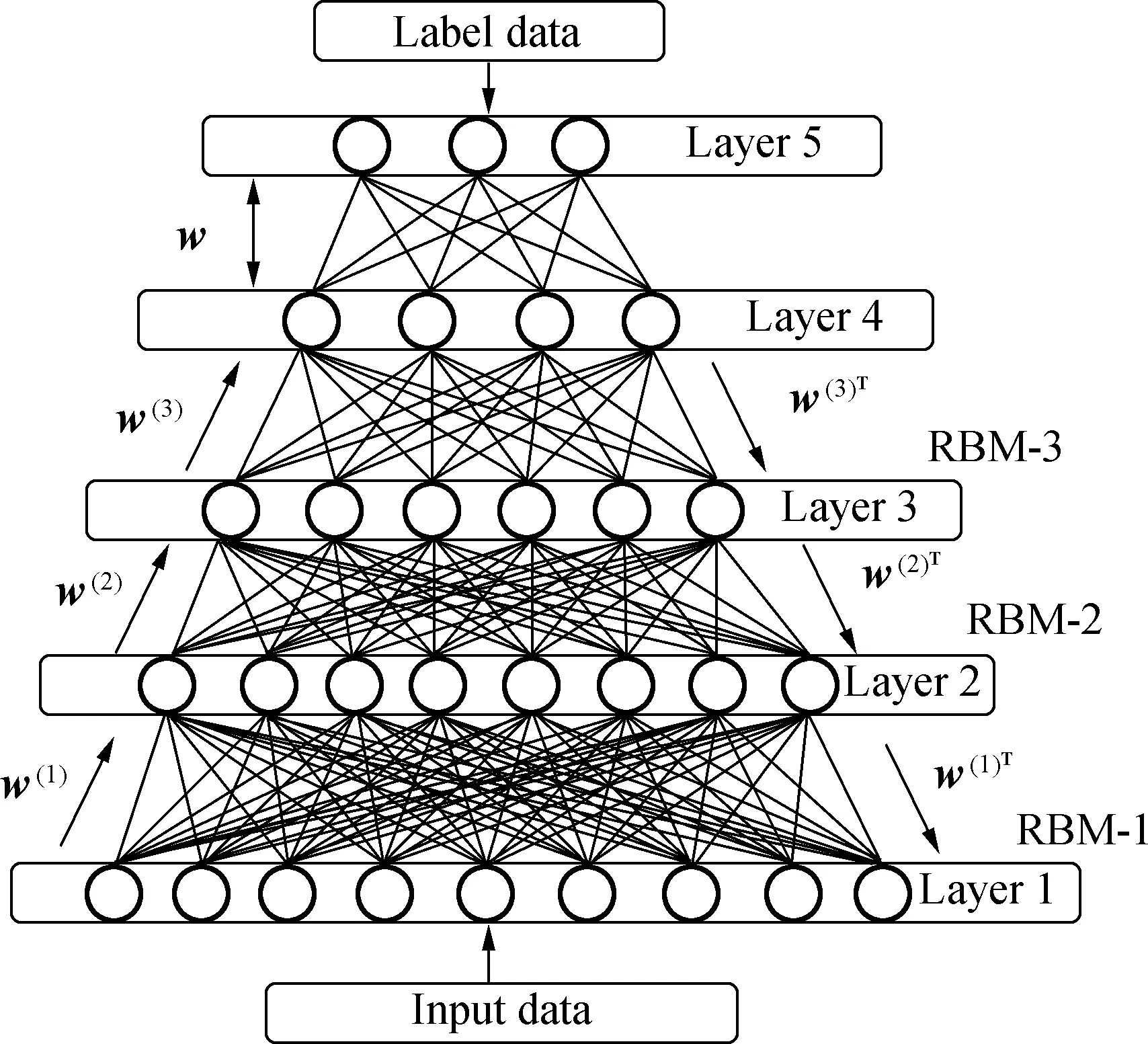
Fig.2 Deep belief network

1.2.1 Layer-by-layer pre-training

In the layer-by-layer pre-training stage, a layer-by-layer training method is adopted to simplify the DBN for the training of multiple RBMs. Assuming that we have trained the RBM of the first 1-1 layer, we can calculate the bottom-up conditional probability of the hidden variable:

P(h(i)|h(i-1))=σ(b(i)+w(i)h(i-1))

(15)

whereb(i)is the bias of thei-th layer RBM andw(i)is the connection weight. In this way, we can combineh(l-1)andh(l)into an RBM. The specific pre-training steps are as follows:

1) Using the original sample as the input, perform unsupervised pre-training on the first layer of the RBM according to the CD algorithm. After completion, fix its weight parameterw(1)and biasa(1),b(1).

2) Learn the hidden layerh(1)of the first RBM through

P(h(1)|v)=P(h(1)|v,w(1)).

3) Use the learned hidden layerh(1)as the input layer of the next RBM, perform unsupervised pre-training on the next RBM according to the CD algorithm, and fix its weight parametersw(2)and biasesa(2)andb(2)after the training is completed.

4) Repeat steps 2) and 3) until the unsupervised pre-training of all RBMs is completed.

1.2.2 Fine-tuning

The specific fine-tuning process is to add another output layer to the last layer of the DBN and then use the backpropagation algorithm to tune the parameters.

2 Numerical Research

2.1 Numerical model

In this study, the finite element model of a steel truss bridge in service in Sweden was established. The Åby Bridge is a steel truss bridge. The steel truss design was used for both bridges and was constructed at the same time. The railway bridge across the Åby River is one of the two bridges, and the other is on the Rautasjokk River. Because the two bridges are used in the same way, the performance of the Rautasjokk Bridge can be roughly estimated based on the field measurements and finite element analysis results of the Åby Bridge.

Under the joint support of the seventh framework project of the European Union,LKAB Iron Mine Company of Sweden, and the Swedish Railway Administration, the research team jointly carried out research studies on the static and dynamic performances of the Åby Bridge with the research team of Luleå University of Technology of Sweden[10]. The research team mainly tested and studied the dynamic response of the Åby Bridge under the excitation of the train load. The bearing distance between the two supports of the Åby Bridge is 33.7 m, the height of the center line of the main truss is 4.7 m, and the distance between the two main trusses is 5.5 m. Along the bridge, it consists of two main trusses and two longitudinal girders. There are transverse connecting members between the longitudinal girders and the main truss. Among them, the transverse connection member between the longitudinal girders is angle steel, while the transverse connection member between the main trusses, in addition to the T-shaped steel member at the bottom, is I-shaped steel that intersects with two longitudinal girders above. I-shaped steel is mainly used in the main truss. The end diagonal bars and upper longitudinal beams adopt closed sections, and stiffening ribs are used at each joint. The actual bridge and three views are shown in Fig.3.

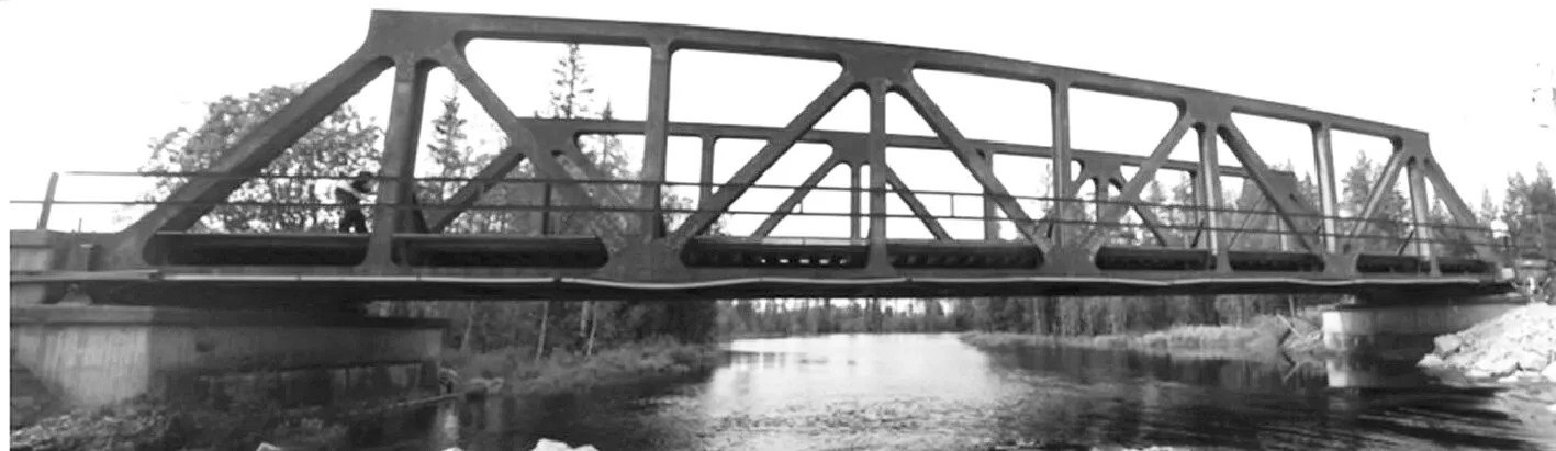
Fig.3 Åby Bridge

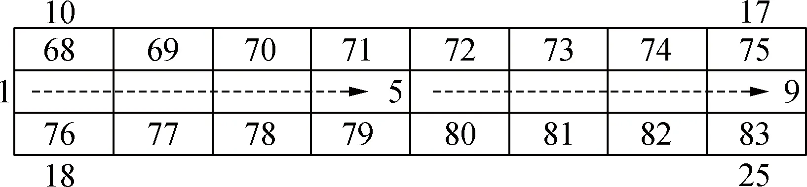
The acceleration response is one of the important indexes to measure the dynamic response of the bridge structure. The site acceleration test points of the Åby Bridge are arranged, as shown in Fig.4, in which the dot is the upper acceleration observation point of the truss, and the star is the lower acceleration observation point.

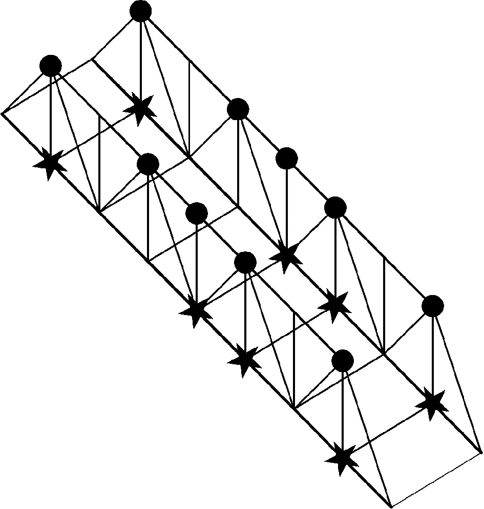
Fig.4 Åby Bridge acceleration test point

The modal and natural frequency extraction of the bridge structure from acceleration measured data using the unweighted principal component random subspace identification method. A finite element model was updated using a response surface model based on multi-objective particle swarm optimization. The density and elastic modulus of the finite element model are used as modified parameters. The elastic modulus and density of the bridge are 200 GPa and 7 800 kg/m3, respectively. After updating the finite element model, the elastic modulus of the Åby Bridge is 191 GPa, the density is 7 785 kg/m3, and the maximum error of the updated frequency is only 2.86% (see Tab.1). In the following research, the updated finite element model can be used as the baseline model to generate training data and verify the performance of the proposed framework in structural damage identification. In the following chapters, the proposed method and ANN will be used to study the vibration characteristics of the damage model. The results of the ANN are compared with the proposed method to prove the superiority of the method.

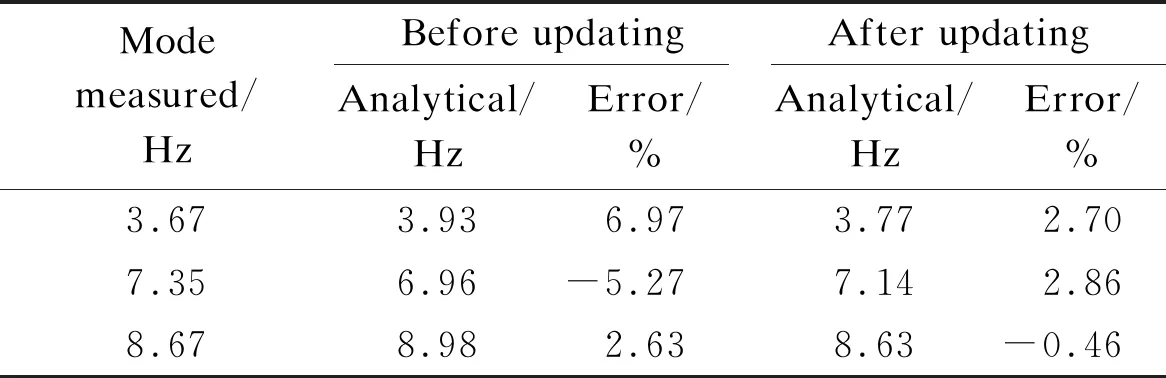
Tab.1 Measured and analytical natural frequencies of the experimental model before and after updating

Fig.5 display the established finite element model. The element type is an Euler beam element. The output is the first five modes in they-axis direction, and the number of modes is 90.

(a)

2.2 Data generation

By randomly selecting two members, the elastic modulus of the specified member was reduced, and the elastic modulus of the other members remained unchanged, which is 191 GPa. A total of 2.6×105samples were generated. To improve the convergence speed and accuracy of the DBN, the input data were normalized, and the deviation standardization was used to normalize the sample data between 0 and 1. The input of the neural network is the first five modal data of the samples, and the output is the damage degree of each member. Considering the influence of noise in the environment, 2% Gaussian white noise was introduced into the modal data. The noise results and non-noise results were compared to study the noise resistance of the proposed model. There are three hidden layers in the DBN, and the units are 120, 100, and 90. For the convenience of comparison, the layers and units of the ANN were set the same as those of the DBN.

(16)

To study the effectiveness and robustness of the proposed method for structural damage identification, the dataset includes the influence of measurement noise and uncertainty in finite element modeling. The following scenarios are defined in the numerical research:

1) There is no measurement noise and uncertainty, and the influence of noise and the uncertainty of finite element modeling were not considered in the dataset.

2) Considering the influence of noise and the uncertainty of modeling, 2% Gaussian white noise was added to the dataset.

3) Without considering the influence of noise and modeling uncertainty,1% uncertainty was added to the stiffness in finite element modeling.

4) Considering the influence of noise and modeling uncertainty, 2% noise was added to the modal data, and 1% uncertainty was added to finite element modeling. The effects of noise and uncertainties are considered for all datasets. Uncertainty was mainly introduced as a 1% variation of stiffness with the Gaussian distribution to simulate the certainty of finite elements.

3 Results and Discussion

3.1 Not considering the impact of environmental noise and modeling uncertainty

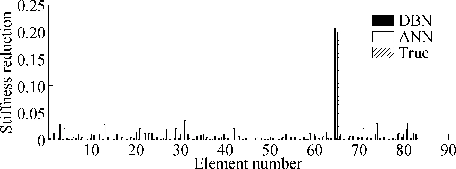
Firstly, considering the damage condition of a bar, the damage degree at position 65 is 0.2. This damage condition is not included in the training center.Fig.6(a) shows that the damage identification results of the ANN and DBN can complete the damage location identification. The result of the DBN identification is 0.207, that of ANN damage identification is 0.182 8, and their absolute errors are 0.007 and 0.017 2, respectively. Hence, the recognition accuracy of the DBN is better than that of the ANN without noise and modeling error.

Secondly, considering the condition that two bars are damaged at the same time, the damage degrees of positions 6 and 46 are both 0.3. This damage condition is not included in the training center. The damage identification results show that the ANN and DBN can complete the damage location identification.Fig.6(b) shows that the damage identification results of the DBN are 0.307 and 0.290, and those of the ANN are 0.384 and 0.163, respectively. Among them, the maximum absolute error of the DBN recognition is 0.01, and the maximum absolute error of the ANN recognition results is 0.137, which means that the recognition accuracy of the DBN is better than that of the ANN without noise and modeling error.

(a)

Finally, considering the damage of three bars, the true damage degrees of No. 3, 16, and 41 locations are 0.2, 0.15, and 0.3, respectively. This damage condition is not included in the training center. Fig.6(c) shows that the damage identification results show that the ANN and DBN can complete the damage location identification. The identification results of the DBN are 0.188, 0.149, and 0.319. The identification results of the ANN are 0.168, 0.105, and 0.228. Among them, the maximum absolute error of the DBN recognition results is 0.019, and the maximum absolute error of the ANN recognition results is 0.072. Hence, the recognition accuracy of the DBN is better than that of the ANN without noise and modeling error.

3.2 Considering the impact of environmental noise

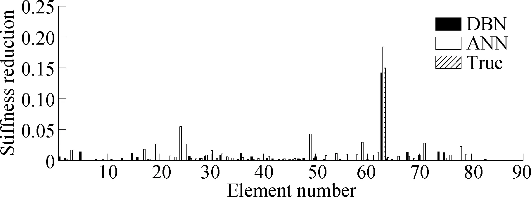
Firstly, considering the damage condition of a bar, the damage degree at position 63 is 0.15. This damage condition is not included in the training center.Fig.7(a) shows that the ANN and DBN can complete the damage location identification. The result of the DBN identification is 0.142, that of ANN damage identification is 0.184, and their absolute errors are 0.008 and 0.032, respectively. Hence, the recognition accuracy of the DBN is better than that of the ANN without noise and modeling error.

(a)

Secondly, considering that two bars are damaged at the same time, the damage degrees of positions 18 and 45 are 0.1 and 0.35, respectively. This damage condition is not included in the training center. Based on the damage identification results, Fig.7(b) shows that the DBN can identify the damage location. The ANN cannot identify the damage at position 18. The ANN can judge position 25, which has not been damaged, as damage. Hence, in the case of ambient noise, the ANN’s recognition accuracy significantly decreases, but the DBN can still complete damage identification.

Finally, considering the damage of three bars, the true damage degrees of No. 4, No. 22, and No. 53 locations are 0.2, 0.3, and 0.15, respectively. This damage condition is not included in the training concentration.Fig.7(c) shows that the DBN can correctly identify the damage location, whereas the ANN cannot identify the damage to No. 53 locations. Hence, in the case of environmental noise, the recognition accuracy of the DBN is better than that of the ANN.

3.3 Considering the impact of modeling uncertainty

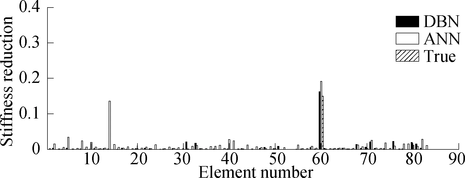
Firstly, considering the damage condition of a member, the damage degree at position 60 is 0.15. The training center does not include this damage condition.Fig.8(a) shows that the ANN and DBN can complete the damage location identification. However, the ANN judges the rod at position 14, which has not been damaged, to be damaged. For the rod DBN at position 60, the damage degree is 0.162. The damage identification result of the ANN is 0.192, and the absolute error is 0.012 and 0.042, respectively, which indicates that the recognition accuracy of the DBN is better than that of the ANN under the condition of the modeling error.

(a)

Secondly, considering the condition that two bars are damaged at the same time, the damage degrees of positions 30 and 65 are 0.2 and 0.3, respectively. This damage condition is not included in the training center. From the results of damage identification, in Fig.8(b), the DBN can identify the damage location, but the ANN cannot identify the damage at position 65. The ANN will identify positions 19 and 25, which have not been damaged, as damaged. Hence, under the condition of the modeling error, the ANN’s recognition accuracy decreases significantly, while the DBN can still complete damage identification.

Finally, considering the damage of the three bars, the true damage degrees of No. 15, No. 32, and No. 61 locations are 0.2, 0.3, and 0.15, respectively. This damage condition is not included in the training center.Fig.8(c) shows that the DBN can correctly identify the damage location, and the ANN cannot correctly identify the damage at No. 61 and the bar at No. 76, which has not been damaged but is judged to be damaged. Hence, under the condition of the modeling error, the recognition accuracy of the DBN is better than that of the ANN.

3.4 Considering environmental noise and modeling uncertainty

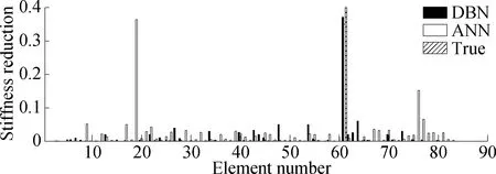
First, considering the damage condition of a member, the damage degree of position 61 is 0.4. This damage condition is not included in the training center.Fig.9(a) shows that the ANN and DBN can complete the damage location identification. However, the ANN judges the position 19 bar, which has not been damaged, as damaged. This finding shows that in the case of environmental noise and modeling error, the recognition accuracy of the DBN is better than that of the ANN.

(a)

Secondly, considering the condition that two bars are damaged at the same time, the damage degrees of positions 15 and 40 are 0.2 and 0.3, respectively. This damage condition is not included in the training center. Based on the damage identification results,Fig.9(b) shows that the DBN can identify the damage location. The ANN cannot identify the damage at position 40, but it can identify the damage at position 61, which has not been damaged, as damaged. This finding indicates that in the case of ambient noise and modeling error, the ANN’s recognition accuracy significantly decreases, whereas the DBN can still complete damage identification.

Finally, considering the damage of the three bars, the true damage degrees of No. 18, No. 41, and No. 69 locations are 0.2, 0.15, and 0.3, respectively. This damage condition is not included in the training center. Based on the damage identification results, Fig.9(c) shows that the DBN can correctly identify the damage location, the ANN cannot identify the damage at the No. 41 location, and the bars at No. 7 and No. 22, which have not been damaged, are judged as damaged. This result shows that the recognition accuracy of the DBN is better than that of the ANN in the case of environmental noise and modeling error.

4 Conclusions

1) The bridge damage identification method based on the DBN can be used to identify the damage location and damage degree of bridge structures. It can also identify small damage under various uncertainties and noises.

2) This method shows a strong anti-noise ability and robustness in the aspect of bridge damage identification. Compared with the BP neural network, this method has more accurate recognition results.

3) The method can use incomplete modal data for structural damage identification and is an effective tool for damage identification.