
Roughness evaluation of three-dimensional asphalt pavement based on two-dimensional power spectral density
2022-02-06 10:54DingZhikeXuFeiyunZhaoXun
Ding Zhike Xu Feiyun Zhao Xun
(School of Mechanical Engineering, Southeast University, Nanjing 211189, China)
Abstract:To solve the problem of the lack of comprehensive evaluation of three-dimensional (3D) asphalt pavement roughness, a method for evaluating the asphalt pavement roughness is proposed based on two-dimensional (2D) power spectral density (PSD). By calculating the 2D PSD of a 3D asphalt pavement and converting it into the longitudinal average asphalt pavement PSD, the relationship between the evaluation method of the 3D asphalt pavement roughness and the current evaluation standard of roughness is established. Combined with the road-fitting formula used in international standards, the elevation data of the A, B, C, and D grades of the 3D asphalt pavement are simulated by the harmonic superposition method. According to the proposed method, the longitudinal PSD of each level of simulated asphalt pavement is calculated and compared with the standard spectral line of each pavement level. This approach verifies the effectiveness of the proposed method in evaluating the roughness of the 3D asphalt pavement. Compared with the PSD of a certain horizontal profile elevation, it is verified that the fluctuation amplitude of the spectral line calculated by the proposed method is greatly improved. The results show that the proposed method can evaluate the roughness of asphalt pavements more comprehensively and accurately and has strong practicability.
Key words:roughness; power spectral density; three- dimensional asphalt pavement
Roughness is one of the main technical indicators for evaluating the quality of asphalt pavements and ensuring driving safety and comfort. The American Society for Testing and Materials defines road roughness as the vertical deviation of the road surface from the ideal plane[1]. Studies have shown that the deterioration and uneven distribution of asphalt pavement quality causes several crash accidents[2], affects driving speed, increases the rolling resistance of driving, accelerates the degradation of automobile parts, and increases automobile maintenance costs[3]. Additionally, uneven asphalt pavement surfaces stimulate vehicles to produce vertical dynamic loads, which are reflected on the asphalt pavements, aggravating the occurrence of asphalt pavement disease.
Among many indicators for evaluating asphalt pavement roughness, the international roughness index (IRI) is the most widely used. Other indicators include the power spectral density (PSD), profile index, and vertical acceleration root mean square[4]. Since asphalt pavement profiles comprise short, medium, and long waves with different characteristics, the roughness characteristics of asphalt pavement profiles can be investigated by analyzing the elevation, velocity, and acceleration variations under different frequencies[5].
Generally,roughness detection technology can be divided into reaction and section types according to the detection principle[6]. It mainly includes the three-meter ruler method, the continuous roughness meter, the hand-push roughness meter, the vehicle-mounted bump accumulator, and the vehicle-mounted laser roughness meter.
With the development of information technology, machine vision has been widely used in several fields, such as robotics and automation, with the advantages of rich information, good timeliness, small size, and low energy consumption[7]. RGB-D sensors[8], binocular vision technology[9], and other technologies are used to obtain more comprehensive three-dimensional (3D) information on asphalt pavement. The transverse and longitudinal sections of 3D asphalt pavements have height changes. Compared with the traditional detection methods, these new detection technologies can obtain the longitudinal and transverse elevation data of asphalt pavement. Conventionally, the calculation method of asphalt pavement roughness is mainly for the longitudinal.
Herein, a new method for calculating the elevation longitudinal roughness of 3D asphalt pavements based on the 2D PSD is proposed. The rest of this manuscript is arranged as follows: Firstly, the roughness index of the PSD and the 3D harmonic superposition simulation method of asphalt pavements are introduced. Next, a new calculation method for evaluating the longitudinal roughness of 3D asphalt pavement elevation is proposed. Furthermore, the 3D asphalt pavements from grade A to D are simulated, and the effectiveness of the proposed method is verified by experimental comparison.
1 Basic Theory
1.1 PSD evaluation of pavement roughness
Several measured data have shown that the elevation of road profiles is generally considered a random phenomenon. In the time domain, it is a stationary random process of all states[10]. As the input of vehicle vibration, the statistical characteristics of road roughness are mainly described by the road PSD. According to the random process theory, the road PSD can be used to analyze the road profile and represent the variations in the variables at different frequencies (wavelengths). Therefore, the unevenness of the road profile can be analyzed by the variations in elevation, velocity and acceleration under different frequencies (wavelengths).
In the 1970s, the International Standard Organization (ISO) proposed the PSD index, which realized the evaluation of road surface profile texture at different scales. According to the road surface spectrum frequency index, road surface roughness is divided into eight grades from A to H in the international standard. In the Road Surface Roughness Representation Method Draft[11]proposed by ISO/TC108/SC2N67, the PSD of the road roughnessGq(n) is expressed as
(1)
wheren0=0.1 m-1is the spatial reference frequency;Gq(n0) is the roughness coefficient corresponding to the road grade;ωis the frequency index, which determines the frequency structure of the road PSD under general conditions, andnis a frequency in the space-frequency effective band. The spatial frequency bandwidth is [n1,n2].
The PSD curve is a spectral density curve with spatial frequency as the horizontal axis and the finite mean square value within the range of unit spatial frequency or spatial angular frequency as the vertical axis. It can represent the distribution of road roughness energy in the spatial frequency domain and describe the structure of road waves. Therefore, it is called the road vertical displacement PSD, or road spectrum for short.
The range and geometric mean values of grade A to H road roughness coefficients are presented in Tab.1, and the frequency index of the graded pavement spectrumω=2. The grading diagram of road roughness is shown in Fig. 1; the graph is expressed in double logarithmic coordinates. The logarithmic coordinates expand the dynamic range of the expression, and the low-power part of the high-frequency end is graphically amplified, whereas the high-frequency power is an important part of the road excitation.
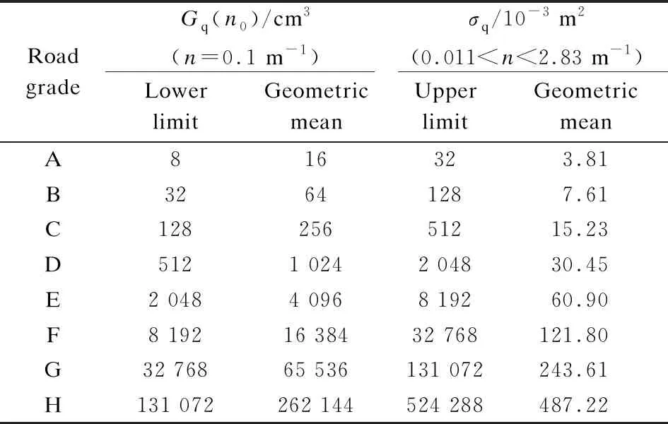
Tab.1 Classification standard for road roughness
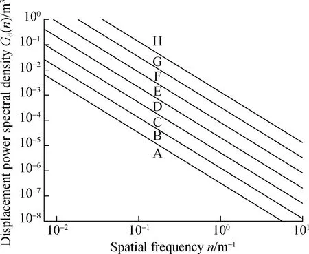
Fig.1 Grading diagram of road roughness
1.2 Harmonic superposition method for 3D asphalt pavement simulation
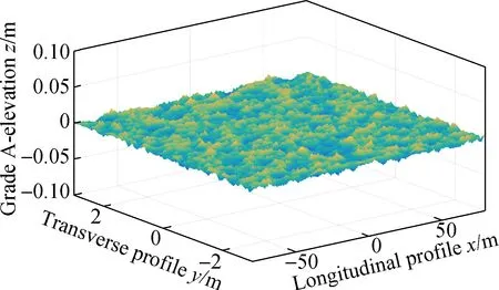
The transverse and longitudinal sections of 3D asphalt pavement have height changes (see Fig. 2), which have an impact on the assessment of roughness. According to the statistical characteristics of the road spectrum, road elevation is a Gaussian process of smooth traversal with a mean of zero. Therefore, different forms of trigonometric series can be used for simulation.
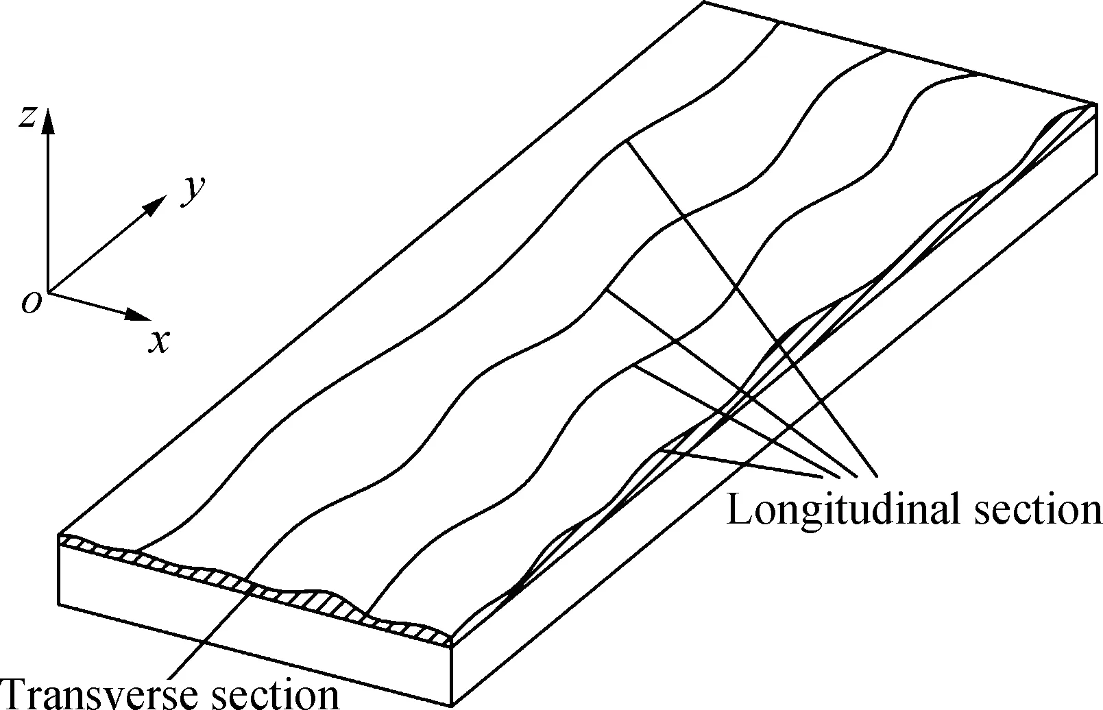
Fig.2 Transverse and longitudinal sections of three-dimensional asphalt pavement
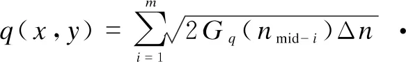
The standard asphalt pavement roughness within a limited range of spatial frequencies can be obtained by the superposition of harmonic components of the asphalt pavement roughness at the central frequency between each partition, as follows[12]:
(2)
wherenmid-iis the central frequency between each cell, wherei=1, 2, …,m;θi∈[0,2π] is a random number with interval uniform distribution; Δnis the sampling interval of the spatial frequency.
To build a random 3D asphalt pavement and increase the elevation distribution of the transverse profile, Eq. (2) needs to be extended, as follows[13]:
(3)
wherexis the longitudinal position of the random asphalt pavement,yis the transverse position of the random asphalt pavement, andθi(x,y) is the random number between [0,2π] of any lineyon the asphalt pavement.
2 Evaluation Method of 3D Asphalt Pavement Roughness
2.1 Two-dimensional PSD of 3D asphalt pavement
In the Euclidean coordinate system, the three-dimensional asphalt pavement can be represented by a functionz(x,y) of two variablesxandy, wherezis the vertical coordinate of the actual surface relative to the theoretical surface height at position (x,y). The two-dimensional Fourier transform ofz(x,y) is given as follows:
(4)
wherefxandfyare the spatial frequencies in thexandydirections; andLxadLyare the lengths of the 3D asphalt pavements in thexandydirections, respectively.
The collected asphalt pavement elevation is discretized. Thus, sampling is performed with sampling pitches Δxand Δyin the spatial region in thexandydirections, respectively, to obtain a spatial surface with a lattice size ofM×N. Then, the spatial frequencies in thexandydirections of the spatial surface are discretized asfp=p/(MΔx)(p=0, 1, 2, …,M-1), andfq=q/(NΔy)(q=0, 1, 2, …,N-1), respectively. Its 2D discrete Fourier transform is given as follows:
0≤p≤M-1, 0≤q≤N-1
(5)
Its 2D PSD calculation equation is expressed as
0≤p≤M-1, 0≤q≤N-1
(6)
To solve the problem of the side lobe leakage in the PSD spectrum, the Hanning window was used for preprocessing. The definition of the 2D Hanning window (normalized window energy) is given as follows:
0≤m≤M-1, 0≤n≤N-1
(7)
The 2D PSD of the 3D asphalt pavement elevation processed by the Hanning window is given as follows:
0≤m≤M-1, 0≤n≤N-1
(8)
2.2 Longitudinal mean PSD
The roughness index mainly reflects the roughness of the longitudinal profile curve. Therefore, it is necessary to convert the 2D PSD into a 1D PSD for the longitudinal pavement evaluation. When the spectrum varies only in a fixed direction, the 1D PSD can be calculated from the 2D PSD. Assuming that thex-direction is the direction of the frequency change, the specific equation is given as follows:
(9)
The discrete form is given as follows:
(10)
Therefore, after the conversion to the longitudinal 1D PSD, the equation is given as follows:
0≤p≤M-1, 0≤q≤N-1
(11)
3 Experimental Verification
3.1 Three-dimensional asphalt pavement simulation
The roughness of the road displacement can be expressed asq=q(l), where the independent and dependent variables are the length and height, both of which are unit dimensions of length. Also,q(l) is the infinite signal in the time domain. In engineering, a section of asphalt pavement with lengthLis usually selected for research. The value ofLshould ensure the spatial frequency resolution. The spatial frequency of the road roughness signal is between 0.011 and 2.83 m-1, so the minimum identification frequency is Δn=1/L≤0.011, that is,L≥91 m.
According to the sampling theorem, the sampling frequency satisfies the condition whenns≥2nmax. Then, the sampling intervals Δxand Δyin thexandydirections should meet the following condition:
(12)
Therefore,Δx≤0.176 7 m and Δy≤0.176 7 m. Herein, Δx=0.1 m, Δy=0.1 m,Lx=160 m, andLy=6 m.
According to Tab.1, the geometric mean value of the grade A road roughness coefficient is selected, and the elevation of grade A 3D asphalt pavement is simulated according to the harmonic superposition method of Eq.(3). Similarly, the corresponding roughness coefficients of grades B, C, and D are selected to simulate the corresponding level of the 3D asphalt pavement elevation according to Eq.(3). The 3D elevation of grades A-D asphalt pavement is shown in Fig. 3.
(a)
3.2 Validity verification
The steps to verify the effectiveness of the method herein are as follows:
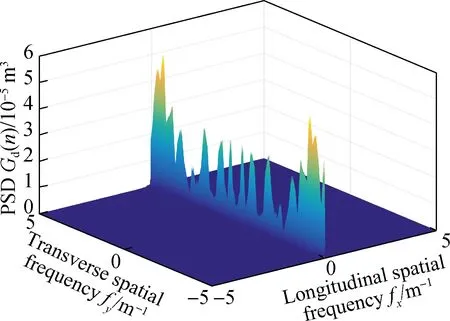
1) The 2D PSD is calculated using the 3D elevation data. According to the elevation data of grades A-D 3D asphalt pavement simulated in Section 3.1, Eq.(8) is used to calculate the 2D PSD of the corresponding elevation data. The 2D power spectral densities of grades A-D asphalt pavements are shown in Fig. 4.
(a)
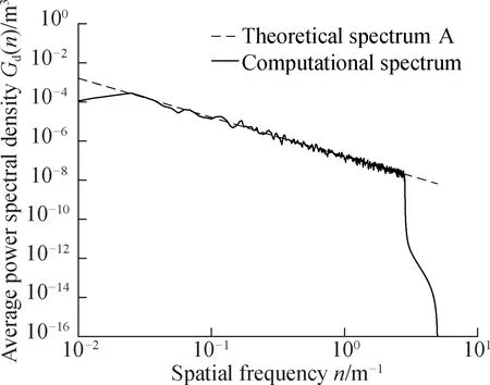
2) The 2D PSD of the 3D road surface is converted into the 1D longitudinal PSD. Since the current roughness index reflects the roughness of the longitudinal profile curve, Eq.(11) is used to calculate the longitudinal 1D power spectral densities of grades A-D.
3) The power spectrum calculated by this method is compared with the standard road spectrum. The 1D power spectrum density spectrum is compared with the corresponding standard pavement spectrum. The comparison results under grades A-D asphalt pavements are shown in Fig. 5.
According to Fig. 5, in the space-frequency range, the PSD lines of grades A-D 3D asphalt pavements calculated by the method herein are very consistent with the standard spectral lines of the corresponding grades. Therefore, the method presented herein is feasible for evaluating the roughness of 3D asphalt pavements.
(a)
3.3 Comparison with traditional methods
According to the national standard[14], the roughness is usually tested using the eight-wheel instrument or the laser roughness profiler as an interval every 100 m to calculate the PSD or IRI of a longitudinal profile. Therefore, the traditional method is used to evaluate the roughness of a profile. Then, to verify the advantages of this method over the traditional method, the PSD of a horizontal profile is calculated and compared with the results of this method.
The comparison steps between the method herein and the traditional method are as follows:
1) The 3D asphalt pavement simulation data in Section 3.2 was selected for experimental verification.
2) The longitudinal 1D PSD of the 3D asphalt pavement is calculated by the method herein.
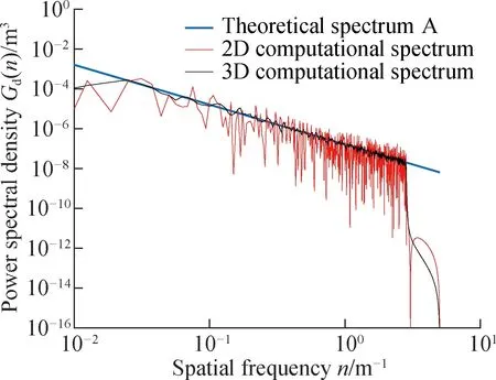
3) The longitudinal section elevation data is selected at the transverse 2 m (y=2 m) of the simulation pavement at all levels, and the corresponding PSD is calculated.
The comparison results with the method herein are shown in Fig. 6.
(a)
The PSD calculated from the elevation data of the transverse and longitudinal profiles fluctuates greatly (see Fig. 6). The PSD spectrum of each grade obtained by this method is very consistent with the standard spectrum of the corresponding grade, and the fluctuation of the spectrum is reduced. The gradient of the standard spectral line is -2. Assuming that the variance of the standard spectral line is zero, the performance index obtained by correcting the spectral line calculated by the traditional and proposed methods is shown in Tab.2. The method proposed herein has a certain degree of improvement compared with the traditional method of calculating the spectral line slope (see Tab.2). In terms of the spectral line fluctuation, the standard deviation calculated by the traditional method is generally 0.8 to 0.9, and the standard deviation calculated by the method proposed herein is ~0.24, with a significant improvement. Therefore, it can be proved that the method presented herein can better evaluate the roughness of 3D asphalt pavements and has high evaluation accuracy.
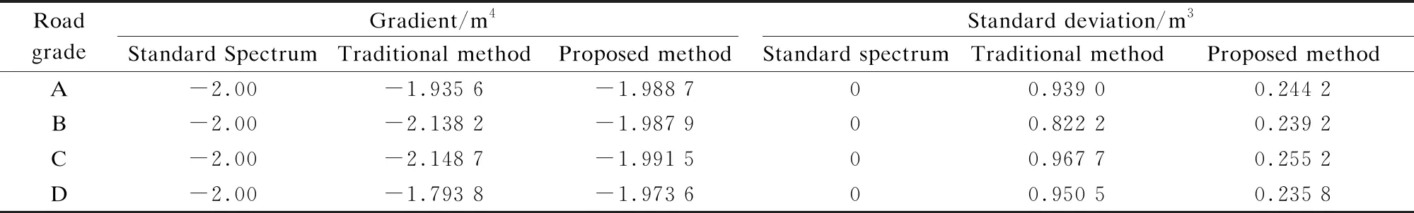
Tab.2 Performance comparison between the proposed and traditional methods
4 Conclusions
1) Based on the elevation data of simulated 3D asphalt pavements, this study finally deduces the equation of the longitudinal average PSD of 3D asphalt pavement by studying the 2D PSD of 3D asphalt pavements to adapt to the evaluation standard of the pavement roughness in the current standard.
2) The simulation case shows that the spectral lines calculated by the method herein are consistent with the standard spectral lines. Besides, the evaluation of the roughness of 3D asphalt pavements is more comprehensive and accurate.
3) The 2D PSD contains the frequency information of the 2D surface and reflects the influence of different wavelengths in different directions. This information is important for evaluating the roughness of asphalt pavements.
 Journal of Southeast University(English Edition)2022年4期
- Journal of Southeast University(English Edition)的其它文章
- WinoNet: Reconfigurable look-up table-based Winograd accelerator for arbitrary precision convolutional neural network inference
- Damage identification of steel truss bridges based on deep belief network
- Deciding whether manufacturing firms share product links on owned social media considering fan effects
- Robust SLAM localization method based on improved variational Bayesian filtering
- Manufacturers’ channel selections under the influence of the platform with big data analytics