Graph dynamical networks for forecasting collective behavior of active matter

Yanjun Liu(刘彦君) Rui Wang(王瑞) Cai Zhao(赵偲) and Wen Zheng(郑文)

1Institute of Public-Safety and Big Data,College of Data Science,Taiyuan University of Technology,Taiyuan 030060,China

2Center of Information Management and Development,Taiyuan University of Technology,Taiyuan 030060,China

3Center for Healthy Big Data,Changzhi Medical College,Changzhi 046000,China

After decades of theoretical studies, the rich phase states of active matter and cluster kinetic processes are still of research interest. How to efficiently calculate the dynamical processes under their complex conditions becomes an open problem. Recently, machine learning methods have been proposed to predict the degree of coherence of active matter systems.In this way,the phase transition process of the system is quantified and studied.In this paper,we use graph network as a powerful model to determine the evolution of active matter with variable individual velocities solely based on the initial position and state of the particles. The graph network accurately predicts the order parameters of the system in different scale models with different individual velocities, noise and density to effectively evaluate the effect of diverse condition.Compared with the classical physical deduction method,we demonstrate that graph network prediction is excellent,which could save significantly computing resources and time. In addition to active matter, our method can be applied widely to other large-scale physical systems.

Keywords: active matter,graph network,improvement of Vicsek,collective motion

1. Introduction

Self-driven clustering is a phenomenon in which individuals form a collective force with regular movement. Individuals cooperate and influence each other to accomplish complex, collective tasks in a self-organized manner that cannot be accomplished by individuals.Individuals will overcome extreme environments[1–5]through collective behaviors of avoiding natural predators, fighting danger, foraging for survival,and collaborating. Such clustered movements are universal in natural groups of microorganisms,insects,animals,etc. (e.g.,microbial clusters,schools of fish,flocks of birds,and so on).Each individual in such a group with the ability to drive themselves is known as“active matter”.[6,7]They generate complex non-equilibrium kinetic phenomena[8,9]that cause processes of phase transition[10]in the system. Extending to human society, the dynamical behavior of active matter in the control coordination and formation control of robot[11]populations,micro-systems, and autonomous multi-intelligent systems[12]helps to explain[13]the generation and change patterns of cluster intelligence behavior. Therefore, how to describe and explore cluster dynamics using theoretical models becomes a crucial proposition.

Among many models for studying cluster motion, the“Vicsek model”[14]is the most classical model with a simple algorithm, which can simulate the natural cluster synchronization phenomenon[15,16]more realistically. The model quantifies[17]the phase transition phenomena in different control modes by controlling the density and noise[18]of particles in the system.[19]Since the introduction of the Vicsek model,scholars in different fields have used it as a base model for improvement and application. The model is gradually diversified and complicated by getting rid of idealization and getting closer to the actual situation of collective motions.[20,21]

However, it is increasingly difficult to use existing dynamical simulation methods to derive the increasingly complex “Vicsek model”:[15]the derivation period is lengthy and the calculation process is complicated when calculating the quantitative criteria of the model, namely, the order parameters. It is also limited to small-scale systems and cannot be extrapolated efficiently to realistic large-scale conditional systems. Nowadays,modern machine learning methods and massive data sets have been widely used in multiple fields[22–24]with increasing capabilities[25,26]of recognition, classification, training and prediction. It can effectively improve the speed and accuracy of problem solving, and is expected to solve some problems that are difficult and impossible to solve by existing inference methods. Therefore, using machine learning techniques[27]and massive datasets to explore classical physics theory[28,29]problems has become popular research currently.

Among many machine learning methods, this study attempts to use the graph network[30]model for learning and prediction. This model has developed from the graph neural networks, combining neural network methods with mathematical methods. It provides a more comprehensive and detailed description of graph network and their inference capabilities and extends and generalizes a multitude of neural network methods. Since the emergence of the graph neural networks in the last decade or so,they have been continuously extended and strengthened[31,32]to involve problems in different domains.[33,34]They have been extended to efficiently solve classical problems[35]using various supervised and reinforcement learning methods. In the physical field,graph neural networks are also gradually becoming involved in studying the physical systems,[36,37]cluster system dynamics,[38,39]active matter,[39–41]etc. The DeepMind team has integrated graph neural networks to propose a “graph network model” that is more efficient than other standard machine learning building blocks[42,43]and has been utilized successfully in many models of physically complex systems.[39,43]Thus,graph network can replace the existing molecular dynamics derivation process to study cluster dynamics specific processes through predictive methods.[44,45]

This study aims to apply a novel machine learning approach to a classical physics problem.[46]We hope to obtain the final state of cluster motion at a specified time step using the predictive capability of graph network models with only the input of initial bit patterns. By this method,we can avoid the complex extrapolation process,effectively save the computational cost,and improve the computational efficiency of the traditional physics models.[47,48]In this study, we construct the graph structure of topological relationships between individuals and neighbors,and predict the sequential covariates by building a graph network model. We analyze the variation in the degree of consistency of the active matter system during the phase transition under different conditions.

2. GN-active model framework

The graph network (GN) model is designed in the form of “end-to-end”,[42]the input and output are both with graph structures that have the same number of nodes and edge structures. Each time we input a set of graphs with the same condition as system parameter. The initial bit pattern is randomly generated and will be different each time. Through training, it is possible to predict the evolution of cluster motion under system conditions. Graph is represented by the tripleG=(E,V,u),Eis the set of edge(reflecting the influence of individuals),E={(ek,rk,sk)}k=1:Ne;Vis the set of nodes(individuals),V={vi}i=1:Nv;uis the global state attribute;Nvis the number of nodes; andNeis the number of edges (ekrepresents the attribute of thek-th edge,rkandskare respectively the receiving node and the sending node,which are the indexes of nodes connected by thek-th edge).

In the Vicsek model, the graph is constructed by visualizing the individual information embedded in the triad. Individuals of active matter are the nodes,containing the speed of motion of active particles and their own positions;the distance and correlation data between particles exist on the edges,and the rate of motion and positions of individuals in the system form the global state. In this study,the number of particles is fixed. Each individual takes itself as the center of the circle,and the individual particle within the circle area of the specified radius is its neighbor node.The correlation between nodes builds edges. The order parameters can be calculated by using the velocity directions of all the particles in the output system,and the global state can be quantitatively expressed.

The computational core architecture of the GN-active model consists of three modules: encoder(GN encoder),core computing block (GN core) and decoder (GNdecoder). The GN-active model frist uses the encoder called GNencoder to encode the input data into particle position,velocity of motion and global parameters (the order parameter that can quantify the degree of system consistency; the predicted model particle number,parameterβ,noise value,system particle density and other related parameters),and compresses the input graph into a potential spatial representation. It is then processed by a GN core block,which is the core computing part of the graph network. The GN core block is cycledNtimes and the information is propagated from a single particle in the Vicsek model to the whole graph, with each cycle achieving one update of the whole graph. The result is decoded by the third module GN decoder and reconstructs the potential spatial representation into another graph. The result still outputs a graph structure with position and velocity information. The specifci process of the GN-active model is shown in Fig.1(a).

In the graph update process of a GN core block,the computation module is divided into three parts: edge, node, and global. Blocks are closely related, and the calculation result of the previous block will become the input of the subsequent block.

During the graph update process, the calculation unit includes six internal functions: three update functions and three aggregate functions. These six functions would update edges firstly, then update nodes, and finally use the updated edges and nodes to update the state of the whole graph, thus completing a graph update. Update function:

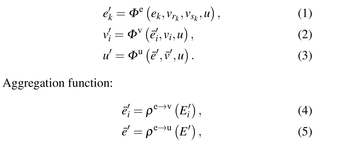
The detailed process of the whole update is shown in Fig.1(b),that is,to realize an update of the graph.

After input the triple structure data of graphG=(E,V,u),the edge block calculates each edge through the edge update functionΦe(formula 1)and outputse′k.The set ofe′kisE′.All edges are polymerized to ¯e′by the aggregation functionρe→u(formula 5),which will work when global status updates.

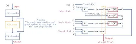
Fig. 1. (a) The core architecture of the GN-active model. The model is divided into three blocks: GN encoder, GN core, and GNdecoder.GNencoder will receive and process input, GN core module will carry out the circular calculation, and GNdecoder will reconstruct the calculation results and output. (b)The GNcore update process of the GN-active model. The update process is divided into three blocks: edge block,node block,and global block,which are node update,edge update,and global update,respectively. The update operation is carried out through the update function and aggregation function.

In the global block, the global attribute will be evaluated by the update functionΦe(formula 3)to yieldu′,where GN outputs the updated set of all edges,nodes,and global attributesG′=(E′,V′,u′).

GN-active model is improved according to the format of the datasets, which can process the Vicsek model data after the optimization of individual speed. Construct the input graph data based on the location direction of active matter.In the whole process of model construction, the input data is frist preprocessed into a graph structure,which is compiled by GN encoder. The working principle of the graph network is shown by Fig.1,in which the GN core cycle update is setup 7 times in order to make the information propagate to the individuals at the edge completely. Finally, the network decodes the generated embedding into the predictedva, which can quantitatively represent the degree of order of the system.After completing the model training,the sequential covariance prediction is specifeid for the test set at the time step. The output predictions are sorted and plotted to show the trend of sequential parametric changes at the specifeid time step during convergence.

3. Results

3.1. Datasets

In fact, in many real clustered systems the individual speed is not constant.In order to further fit the reality,the standard Vicsek model needs to be optimized for individual speed,i.e., individual speed that changes with adjustable parameter;while other conditions remain unchanged, determined the individual’s own speed by the environment around. The velocity is adjusted according to the local order parameters of the neighbor individual’s direction of motion, so that the Vicsek model is no longer the simplest and most ideal model.[42]

To effectively measure the orderliness of the system, we still refer to the order parameter to reflect the consistency degree of the whole system.The order parameter can be obtained according to

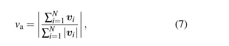
whereviis the individual velocity of the active matter. In this improved model, the speed and direction of each individual are variable in each time step;vais between 0 and 1, and we only consider the direction of velocity.Whenva=1,the active matters in the system are ordered. Whenva=0,the system is unordered(random direction).

In the standard Vicsek model,the velocities of individual particles only change direction. Different from the standard Vicsek model, the speed and direction of individual particles are variable and affected by local order parameters. The updating formula to determine the speed is[12]

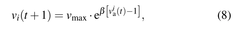
whereviais the local order parameter within the circular range taken by the active particle with itself as the center and fixed radiusR, which is used to quantify the consistency of local particles. The parameterβcan adjust the variation trend of individual speed. Whenβ=0,formula(8)is consistent with the Vicsek standard model(vmax). Whenβ ＞0,the local consistency of the individual is higher, the particle moves faster,which promotes faster synchronization of the system.

Thus,the individual speed can basically reflect the degree of order within the specified radius. In formula(8),when the degree of consistency is high, thevi(t+1)tends tovmax, and the individual moves at the maximum speed set. When the degree of consistency is low, thevi(t+1) tends to 0, and the individual basically lingers.

We use python to design iterative programs to calculate the sequential covariates within a specified radius area centered on each individual. Thus, the speed at the next time step of that individual is updated. We designed simulations ofN=300 particles in anL×Lregion under two-dimensional periodic boundary conditions for active matter dynamics. The initial velocity of each individual is set as 0.03,the parameterβtakes 0, 0.1, 0.5, 1, 2, 5, 10, noiseηis 0, 1, 2, 3, 4, 5, 6,and the length of the simulated box sideLis 5, 10, 15, 25.By setting different environmental parameters,the advantages and disadvantages of the prediction results under different circumstances have been analyzed.

We have trained the models under these environmental conditions, generating 100 independent datasets for each of these conditions as training datasets, and regenerating 100 datasets as test datasets for evaluation of the models. Under each condition,there are 100 sets of training data and 100 sets of prediction data,each group will haveTtime steps,and theXandYaxis position and direction data ofNparticles. Meanwhile,we also calculated the system order parameters of each time step.

3.2. Optimal parameter β

In order to observe the effect of parameterβand to analyze its influence, we observe the individual motion of specified time and step under differentβ, and look for the direct influence ofβchanges on the cluster.

As can be seen from Fig.2,when the value ofβis larger,the order of magnitude of the difference between the velocity of individuals with high and low velocities is greater. It can be observed that individuals with high-speed show longer lengths in the configuration diagram, and individuals with low speed are closer to the“node”shape. Therefore, it can be seen that their speed is approaching 0,and the individual is in a“hesitation”state.

At the same time,with the increase ofβvalue,there will be more clusters moving in different directions.These clusters will easily change each other’s direction when they meet in the process of moving. The time required for the consistent convergence of the whole system is longer. At the same time,the larger theβvalue is,the more difficult it is for the curvilinear motion to appear in the system. It can even be observed that the two cluster directions are opposite to each other.The direction of the cluster with a small number of individuals will be changed,and the individuals in the area where the two clusters conflict in the first place will gradually slow down to 0, and then move back into the larger cluster.

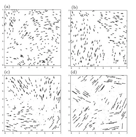
Fig. 2. Motion configuration rendering of the Vicsek model for individual speed optimization. Set L=7,N=300,η=0.1,and R=1 as the condition is fixed when the β values are 1, 5, 10, and 20, respectively. In the period before convergence,the configuration diagram at the 10-th step has selected to observe the influence of β change on the configuration change. (a) The configuration diagram of step 10 under the condition of L=7, N =300,R=1,η =0.1,β =1. (b)The configuration diagram of step 10 under the condition of L=7,N=300,R=1,η =0.1,β =5. (c)The configuration diagram of step 10 under the condition of L=7,N=300,R=1,η =0.1,β =10. (d) The configuration diagram of step 10 under the condition of L=7,N=300,R=1,η =0.1,β =20.

In order to control the variableβin the subsequent prediction and analyze the effects of other parameters on the system,the effects of differentβvalues on the convergence of the system need to be defined first.

Figure 3 shows that with the increase ofβ,we calculated and recorded the time steps for completing convergence under differentβconditions and draw this graph accordingly. In this simulation process,the average value of the order parametervain the last 200 time steps is obtained from the 1000 time steps after the curve is stable.When thevaof the system reaches this mean value for the first time in the process of moving,it is the“convergence time step”. The convergence timeTdecreases first and then increases,and the bestβmakes the convergence speed fastest and the convergence time shortest. In this graph,β,which makes convergence fastest,exists at about 1.0.

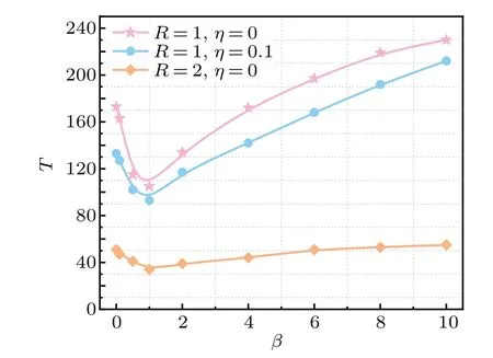
Fig. 3. Finding the optimal parameters β. Set L=7, η =0.1, R=1,change η and β,compare and observe the change of the step value when convergence.

Therefore, we fixedβ=1, based on the fastest convergence speed, generated the initial configuration under different conditions,and transformed it into a graph network. Then we carried out theNtimes of the graph update process in the model and got the prediction results under different parameters.

3.3. Specific applications of prediction

3.3.1. Parameter β affecting speed

In order to observe the prediction ability of the model,we first use the datasets with differentβvalues to conduct training prediction, compare the prediction with the true value curve,and explore the prediction effect after changing parameterβ.

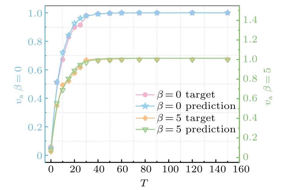
Fig.4.Parameter β simulation results.Under the condition of changing parameter β,the blue line is the actual value of the combined velocity va, and the orange line is the predicted value of the combined velocity va. (a) N =300, L=5, R=1, η =0, β =0, which is the comparison between the predicted and the true value under the standard Vicsek model. (b) The comparison of N =300, L=5, R=1, η =0, β =5.Curve is the fitting of va values obtained when the time step takes 0,5,10,15,25,30,35,40,45,50,55,60,75,90,120,and 150.

According to the curve comparison in Fig.4,the prediction effect is still excellent even if theβvalue changes to a certain extent. The difference ofβleads to different convergence efficiency of the system.Under the same noise condition,even

though the convergence time is obviously different, the order parametervaafter convergence tends to the same value.

3.3.2. Analyzing the noise η

By changing the noiseη,the influence of variation of the parameter noise on the accuracy of the prediction results of the graph network has been observed. In the datasets parameter design, the control variableβshould be discussed at 1.0 when the value ofβis no longer the variable in question.

As can be seen from the curve comparison in Fig.5,whenηis smaller,the fitting degree of the two curves is higher. The prediction curve after increasingηvalue has obvious fluctuation,while the prediction effect is still excellent:the prediction curve is still in the fluctuation range,and the fluctuation range is much smaller than the true value curve. With the increase ofη, the order degree of the system will be greatly affected, so the accuracy of the prediction results will be greatly affected.

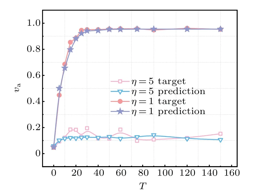
Fig.5. Noise variation simulation results. Set N=300,L=5,R=1,β =1,change the predicted and true values of the noise η=1 and η=5 under the condition,and take the fitting of va values obtained at the time steps of 0,5,10,15,25,30,35,40,45,50,55,60,75,90,120,and 150.

3.3.3. Adjusting the density ρ

In order to further verify the predictive power of the model, the system region side lengthLhas been changed to vary the individual density in the system(Fig.6). We hope to observe the ability of prediction and other interesting phenomena in this way.

In Fig. 6 it can be observed under the condition that the noiseηand parameter values are fixed, the prediction curve gets influenced by side lengthLchanging. WhenLgradually becomes larger,and the number of individuals existing in the system does not change,the density is reduced gradually. This may show that the neighborhood,around which each individual will reduce communication between individuals, will be greatly affected,leading to a much slower convergence speed and significantly increased convergence time. Also, the increase ofLreduces the density of the system and leads to its instability. In that case,the prediction accuracy is reduced,but the overall prediction accuracy of the graphical neural network still stays at a high level.

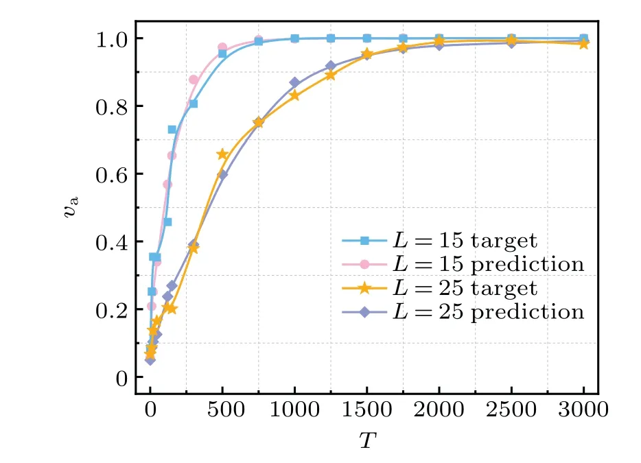
Fig. 6. The simulation results in density change by modifying side length L.Under the fixed conditions N=300,η =0,β =1,the curve of va convergence between the real value and the predicted value has been observed.

4. Conclusions

Our simulation results show that the graph network constitutes a powerful tool to predict the long-term dynamics of active matter, leveraging some of the structure hidden in the local neighborhood of particles. The graph structure is used to describe the relationship between individuals. The graph network trains the model by learning the process of particle position and orientation changes in the system to predict the effect of different environmental settings on the global attribute order parametervaand to find the optimal influence parameters.Thus,the influence of global attribute order parametervaunder different environment settings is predicted,and the best influence parameter is found. We hope that through this method,machine learning can be used to complete the deduction and prediction of large-scale physical systems, and can even be extended to the prediction and interpretation of systems under special conditions.

Active matter systems can generate large and high-quality datasets, which can correspond to complex but controllable physical phenomena that do not require any prior on the relevant physical quantities of the underlying system. Vicsek is an idealized model.Based on this model,this study optimizes the individual velocity close to the reality, so as to make a more realistic and reasonable explanation for the results. We hope to set up more improvements to the Vicsek model to make it more realistic.Datasets with different parameters are designed for training and prediction,and the influences of different variables on prediction results are explored. Each training starts from the input end to the specified time step as the output end,so continuity inference cannot be carried out. Therefore, it is still necessary to deepen the understanding and improvement of the GN-active model and explain the internal process of this “end-to-end” model. At the same time, it is also hoped that new quantitative parameters can be found in the research process to judge the cluster state in the system phase transformation process from different angles. In the process of studying and improving the graph network model, we will apply this model to other complex physical systems and predict more special and large-scale system inference effects.