
Application of Galerkin spectral method for tearing mode instability
2022-11-21 09:28WuSun孙武JiaqiWang王嘉琦LaiWei魏来ZhengxiongWang王正汹DongjianLiu刘东剑andQiaolinHe贺巧琳
Chinese Physics B 2022年11期
关键词:孙武
Wu Sun(孙武) Jiaqi Wang(王嘉琦) Lai Wei(魏来) Zhengxiong Wang(王正汹)Dongjian Liu(刘东剑) and Qiaolin He(贺巧琳)
1College of Physics&Key Laboratory of High Energy Density Physics and Technology,Sichuan University,Chengdu 610065,China
2School of Physics,Dalian University of Technology,Dalian 116024,China
3School of Mathematics,Sichuan University,Chengdu 610065,China
Magnetic reconnection and tearing mode instability play a critical role in many physical processes. The application of Galerkin spectral method for tearing mode instability in two-dimensional geometry is investigated in this paper. A resistive magnetohydrodynamic code is developed, by the Galerkin spectral method both in the periodic and aperiodic directions.Spectral schemes are provided for global modes and local modes. Mode structures, resistivity scaling, convergence and stability of tearing modes are discussed. The effectiveness of the code is demonstrated, and the computational results are compared with the results using Galerkin spectral method only in the periodic direction. The numerical results show that the code using Galerkin spectral method individually allows larger time step in global and local modes simulations,and has better convergence in global modes simulations.
Keywords: Galerkin spectral method,tearing mode instability,magnetic reconnection,magnetohydrodynamics
1. Introduction
Magnetic reconnection,the topological rearrangement of magnetic field lines, was proposed to explain solar flares by Giovanelli.[1]In astrophysical,[1–5]space,[6–9]and laboratory plasmas,[10–14]the phenomenon has been broadly observed, which converts the magnetic energy into thermal and kinetic energies of the plasma. Theoretically, there are two widely quoted theoretical magnetic reconnection mechanisms,namely Sweet–Parker model and Petschek model.[15,16]Magnetic reconnection is considered to play an important role in some processes, such as the solar flares,[2,17–21]the corona heating,[3]the coronal mass ejections (CMEs),[22]the magnetic substorms[23]and the disruption in tokamaks.[24,25]For solar flares, the CSHKP model is regarded as a standard model, in which the conversion of magnetic energy during the magnetic reconnection is thought to provide an origin for the released energy of solar flares.[17–20]Meanwhile, the extreme ultraviolet and x-ray observations also provide evidence of magnetic reconnection in solar flares.[21]In Earth’s magnetosphere, the magnetic substorms explosively release energy from the solar wind, and magnetic reconnection at the magnetotail is considered to be responsible for the magnetic substorms.[23]Magnetic reconnection can be triggered by tearing mode instability, which results in magnetic islands as a consequence of finite resistivity. As one of the important magnetohydrodynamics (MHD) instabilities, tearing mode instability has been widely observed in toroidal plasmas. The magnetic island can be driven by the nonlinear tearing mode,and causes energy loss,crash and disruption.[25]As a catastrophic loss of plasma control in tokamaks, the disruption leads to large heat loads and mechanical stresses on surrounding structures,even causes damage to the machine.[25]Hence,it is crucial to develop the theoretical and simulation study of the tearing mode instability so that the dynamics of many related processes can be well understood. The linear and nonlinear theories of the tearing mode were developed by Furthet al.[26]and Rutherford.[11]
Spectral methods which originated in Ritz–Galerkin methods consist of Galerkin,tau and collocation methods.[27]The main difference between spectral methods,finite element methods and finite difference methods is that spectral methods use infinitely differentiable global functions as the trial functions to approach the solutions. The most frequently used trial functions are orthogonal polynomials. Spectral methods are global because the computation at any point depends on the information from the entire domain. The significant feature of spectral methods is that the convergence could be more rapid than any finite power of 1/N, whereNis the number of the terms in the orthogonal polynomials, while the solution is infinitely smooth.[27]Many schemes of spectral methods have been developed in the last few decades, especially in computational fluid dynamics.[27–29]Applications of spectral methods show good performance on many problems,such as compressible flows, incompressible flows, boundary layers, parallel flows and turbulence flows. For example, Serre and Pulicani proposed a high accuracy pseudospectral method for the computation of the three-dimensional Navier–Stokes equations inside a rotating cavity and the results have a good agreement with experimental and numerical studies.[30]
In recent years, several MHD codes have been developed, such as NIMROD,[31]XTOR,[32]and CLT,[33]which have been widely used to study tearing modes. Finite element and finite difference methods are used frequently as the discrete forms in these codes. Spectral methods are also used in periodic directions, showing a good performance. For instance,NIMROD uses a Fourier representation in the toroidal direction, while the accuracy for derivatives in that direction is increased and several numerical tasks are eased. XTOR uses it in all the angular directions, and the linear algebra is much more efficient for the same spectral content.Another 3D MHD code CLT,developed in recent years,also uses spectral methods in theφdirection of a cylindrical coordinate system(R,φ,Z). The effectiveness of these codes has been demonstrated, and many physical problems were studied by using these codes.[34–39]Hence, the applications of spectral methods are noteworthy in MHD simulations of tearing mode instability. However,it seems that spectral methods are not used as the discrete form individually. For example, XTOR uses a finite difference method in the radial, NIMROD uses a highorder finite element method in the poloidal plane,which uses spectral elements with high-order basis functions inside each element. In these codes, Fourier representations are used in one or two directions,and the computations are performed in the spectrum space and the physical space.
This paper investigates a Galerkin spectral method for simulating tearing modes based on a 2-field reduced magnetohydrodynamics (RMHD) model in two-dimensional space.The main feature of our code is that the Galerkin spectral method is used both in periodic and aperiodic directions.Thus,computations are performed in the spectrum space, and we do not need to transform polynomials into values, or vice versa. The mode analysis and filtering are also more convenient. Three cases are simulated in this paper,namely,case I,II,and III,which represent the single tearing mode,the double tearing mode and them=1 global tearing mode with a slab geometry,respectively. This paper is organized as follows. In Section 2, the physical model we used is given. We present the numerical algorithm in Section 3. Section 4 presents the simulation results and influences of using spectral methods individually. In the final section,a brief conclusion is given.
2. Physical model
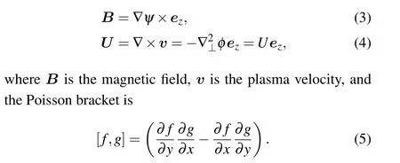
In this paper, a rectangular coordinate system (x,y) is used. For the MHD instabilities, especially the finite resistivity induced tearing mode, the system can be described by the resistive MHD model. In the slab model, the plasma is assumed to be equilibrium static so that the initial plasma velocityv0=0, and the plasma mass densityρis invariant because the flow is incompressible. For simplicity,ρis considered constant:ρ=1. The set of fundamental equations are given as follows:[40]

whereψ,φ,S,U, andjz=-∇2⊥ψare the magnetic flux function,stream function,Lundquist number,vorticity,andzcomponent of current density, respectively. The functionsψandUcan be expressed as
The Lundquist numberS=τη/τa,whereτη=μ0L2/ηis the diffusion time due to the finite resistivity andτa=L/vais the Alfv´enic time. The characteristic lengthLis twenty times the current sheet width,va=BL/(μ0ρ)1/2is the Alfv´enic speed,BLis the magnetic field atx=L,μ0is the vacuum permeability, andηis the plasma resistivity. Variables are normalized asv/va→v,t/τa→t,B/BL →B,E/(vaBL)→E,J/(BL/μ0L)→J,ψ/(BLL)→ψ,φ/(vaL)→φ,U/(va/L)→U,andη/(μ0L2/τa)→η,whereEandJare the electric field and current density,respectively.
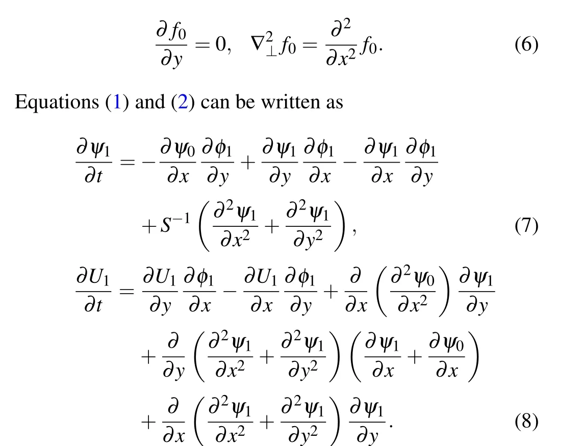
By asymptotic expansion method, a functionfcan be represented asf(x,y,t)=f0+f1(x,y,t), where the subscript 0 and 1 denote equilibrium quantities and perturbations, respectively. For the equilibrium quantities independent ofy,we have
3. Numerical algorithm
In this MHD code,Galerkin spectral method is employed in all directions, and the 4th order Runge–Kutta scheme is used in the time-advance. The simulation domain is (0,b)×(0,c). Because Galerkin spectral method is used in all directions,computations are performed in the spectrum space.
In Galerkin spectral method, the trial functions must fit the boundary conditions, and the test functions are the same as the trial functions. In this paper,the simulation includes local modes and global modes. Fourier functions are used as the trial functions in theydirection because of the periodic boundary conditions. Different boundary conditions were assumed according to the features of local modes and global modes.
For case I, the plasma displacement of single tearing mode is localized around the rational surface,[41]thus the perfectly conducting wall boundary can be applied in thexdirection. For case II,the double tearing mode can exist when two rational surfaces are close enough.[41]Away from the rational surface, the perfectly conducting wall boundary condition is still suitable for case III.
For cases I and II, half-wavelength sine series is used to fit the boundary condition,and the perturbed field can be represented as
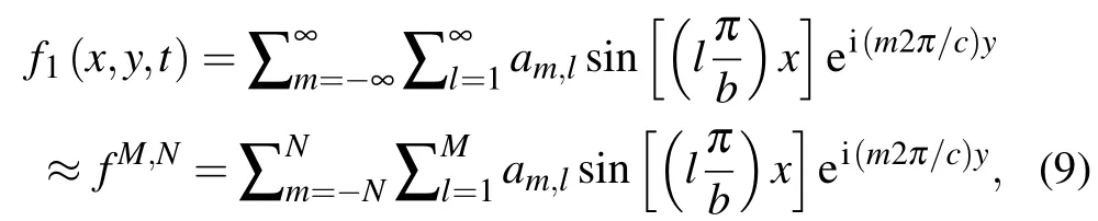
wheream,lis the coefficient,which is also the amplitude of the corresponding Fourier(m,l)component,wheremandldenote the mode numbers inyandxdirections.
The trial functions and test functions can be chosen with above equations. In the Galerkin spectral method, equations(7)and(8)become

wherefM,Nis the conjugate offM,N, equilibrium quantities and perturbations are represented as trial functions.
With the orthogonality of the trial functions and test functions,equations(12)and(13)can be transformed to coefficient equations. Thus, the differential equations(7)and(8)can be solved in the spectrum space, and the derivations of coefficient equations are shown in the Appendix B.The coefficients of the stream functionφcan not be obtained directly,and it is necessary to solve Poisson’s equation at every time step. Fortunately,Uis represented by polynomials in this paper. Thus,the Poisson’s equation becomes a linear equation of the two coefficient vectors.
To compare with the Galerkin spectral method, we also implement finite difference collocation method.The code uses the finite difference method in thexdirection and the Fouriercollocation method in theydirection. The computational grid is vertically divided, and each term of sine series or cosine series in the Galerkin spectral code corresponds to one node in the finite difference collocation code. In theydirection,the fast-Fourier transform(FFT)is used to transform fields to Fourier functions, where derivation is easily computed, then the inverse FFT transforms the results back into the real coordinate space. The Poisson’s equation ofUis solved by transformingUinto a suitable function ofxandy.
4. Simulation results
In this section, the simulation results of the three cases are shown. By comparing with the linear theory,the effectiveness of the Galerkin spectral code is implemented. Then the influence of using the Galerkin spectral method is discussed by comparing the results of the Galerkin spectral code with the finite difference collocation code.
4.1. Equilibrium and perturbation setting
The simulation region is(0,1.5)×(0,1). The set of equilibrium magnetic field is

wherexqis the peak position of the current sheet anddis the sheet width. We choosed=0.05. For case I,xq=0.75. For case II,xq=0.3.
For case II,there are two current sheets,so the magnetic field is given by

wherexq1andxq2are the peak positions of two current sheets,xq1=0.72,xq2=0.78.
The initial perturbation is set as
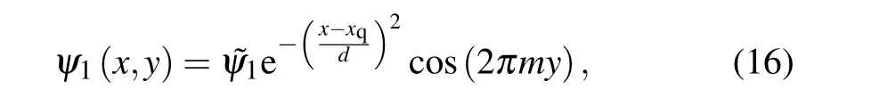
wheremis the mode number in theydirection and ˜ψ1is the amplitude of the initial perturbation.
The equilibrium parameter settings of case I, including the magnetic fieldB0, the magnetic fluxψ0and the current densityj0,are shown in Fig.1(a). As the trial functions have been chosen in Section 3,B0andj0can be transformed into truncated cosine series and sine series,respectively.
The global modes also have been simulated. If there is more than one rational surface(k·B=0)and these surfaces are sufficiently close, the double tearing mode can exist because of the drive between each rational surface.[41]Thus,the equilibrium of case II has two close current sheets, as shown in Fig.1(b). Case III is simulated with suitable boundary conditions chosen in Section 3, and the equilibrium is plotted in Fig.1(c).

Fig.1. Equilibrium profile of the three cases: (a)I,(b)II,and(c)III.
4.2. Mode structure
Figure 2(a) shows the mode structure of a linear single tearing mode. According to the Furth–Killeen–Rosenbluth(FKR)theory,[26]the mode is purely growing and symmetric.Priest showed the mode structure of the linear tearing mode in his paper,[24]which is in accordance with the result.
The result of case III is reported in Fig.2(b). Them=1 tearing mode in cylindrical geometry is found when the safety factorq <1 at the center of the plasma, which results in a displacement of the entire plasma column instead of significant distortions of the flux surfaces.[42]The mode structure in Fig.2(b)shows the rapid decrease of the magnetic flux in the current sheet. Thus,case III is also tested.
In Fig. 2(c), the linear result of case II is plotted, with a small surface distance. The mode structure of a large rational surface distance is shown in Fig.2(d). As the two graphs show, the two single tearing modes developed at each corresponding rational surfaces couple with each other when they are close enough. When the distance is sufficiently large, the modes decouple, and the double tearing mode becomes two single tearing modes.
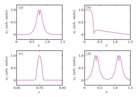
Fig.2. Mode structures: (a)case I with S=106, (b)case III with S=105,(c) case II with S =106, (d) case II with S =106 while xq1 =0.375 and xq2=1.125.
4.3. Resistivity scaling of growth rates

The scaling benchmark of the Galerkin spectral code and the finite difference collocation code are shown in Fig.3. The data are plotted in the double-logarithmic coordinates,and the theoretical scaling is plotted as a line. The scaling results of these two codes are in good agreement. In Fig.3(a),the scaling of growth rates of case I is shown,and the resistivity scaling is nearS-3/5over the range ofSfrom 105to 107. Figure 3(b)shows the result of case II,and the accurate range ofSis from 5×10⁶to 107. The scaling of case III plotted in Fig.3(c)shows that the data provides a good fit to the theory whenSis near 105. Thus,the scaling results of the three cases are all in accordance with the theory.
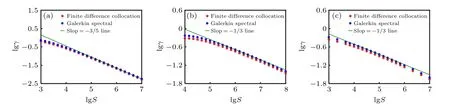
Fig.3. Resistivity scaling of growth rates for the three cases: (a)I,(b)II,and(c)III.
4.4. Convergence benchmark
The convergence in thexdirection is benchmarked in this part. As the spatial resolution increases, the data error of a numerical code should converge to zero.
Figure 4 shows the growth rate convergence of the two codes under the same spatial resolutions, while the resistivities are chosen based on the scaling result. In Fig. 4(a), the convergence rates of the two codes are similar. For case II or III, it shows a significant difference that the convergence of the Galerkin spectral code is faster compared to the finite difference collocation code. As shown in Fig.4(b),the Galerkin spectral code reaches convergence when the number of grid points is larger than 600, while the convergence of the finite difference collocation code needs a larger grid number. For case III,the result in Fig.4(c)reveals much difference. Thus,the simulation indicates that the Galerkin spectral code has a better performance of the convergence in global modes simulations,which shows better accuracy.

Fig.4. Convergence comparisons: (a)case I with S=106,(b)case II with S=106,(c)case III with S=105.
4.5. Stability analysis
The time step is limited by the numerical stability. Figure 5 shows the limited maximum time step of the two codes.The maximum time step Δtis compared under equal grids,and the resistivities are chosen based on the scaling result. As Fig.5(a)shows,the results of case I and II are the same. Compared with the finite difference collocation code,the Galerkin spectral code allows larger time step at small grid number,and Δtdecreases faster as the grid number increases.
As the results in Fig.5(b),the maximum time step shows a relationship nearly Δt∝n-2with the grid number, so further computations are performed. In Fig. 6(a), the maximum time step of case I and II withS=104are shown. The smaller resistivity is chosen because of less computational cost, and there is still a square relationship. The influence of the timeadvance scheme is also discussed in Figs. 6(b) and 6(c), the relationships between Δtandnunder different schemes are sufficiently close.
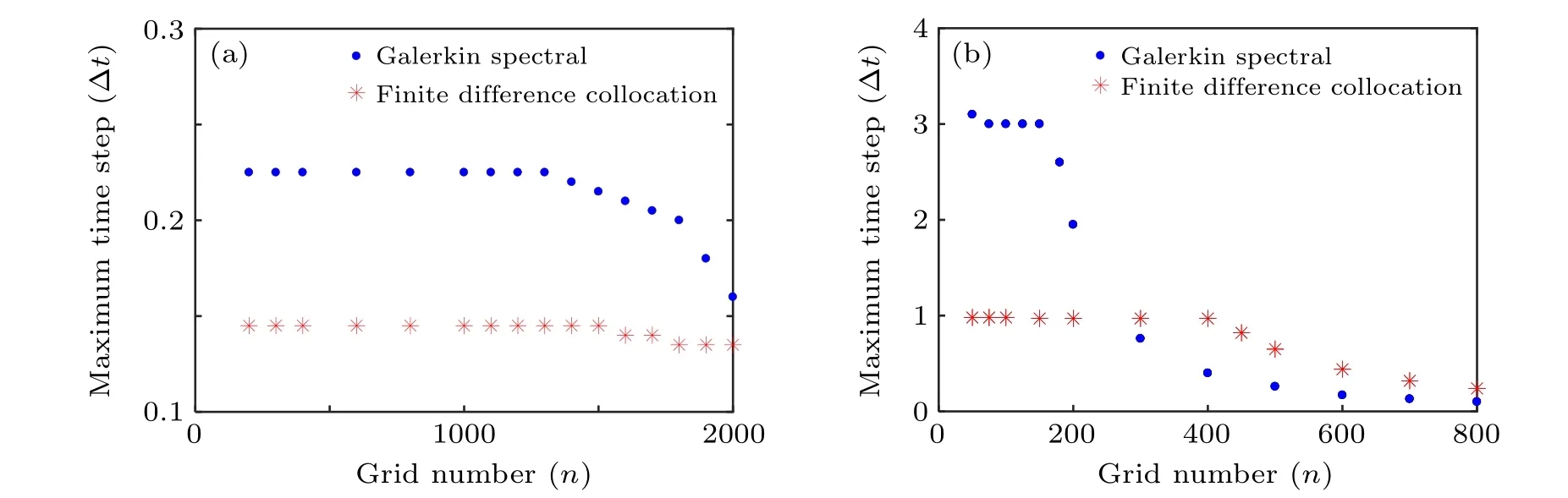
Fig.5. Maximum time step comparisons: (a)the same result of case I and II with S=106,(b)the result of case III with S=105.
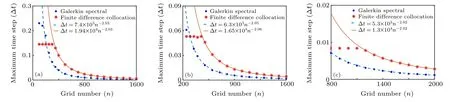
Fig.6. Maximum time step of case I and II with S=104: (a)4th order Runge–Kutta method,(b)2nd order Runge–Kutta method,(c)Euler method.
4.6. Nonlinear results
Considering the fine mode structure of tearing mode inxdirection,the nonlinear simulation of the single tearing mode is performed with-8≤m ≤8 and 1≤l ≤256. Because the boundary conditions are based on local modes,them=1 mode in this case is equal with them ≥2 modes in the cylinder geometry. The nonlinear simulation uses the same equilibrium profiles as that in case I, which is shown in Fig. 1(a). The perturbation is set as Eq.(16).

Fig.7. Growth of magnetic flux perturbation in the current sheet.
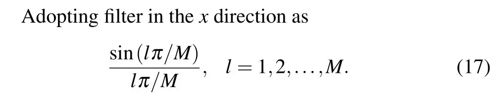
The filtering is performed by altering the expansion coefficients so that the expansion coefficients decay faster for the higherl.The computation is convenient because the equations are solved in the spectrum space.
Figure 7 shows the magnetic flux perturbation,including modes from 0 to 8 and the sum of all modes.Them=1 perturbation drives the increase of highermmodes,and the growth is exponential in the linear stage. As the higher harmonic grows,the nonlinear interactions between different modes become stronger, and the exponential growth is drastically slowed in the nonlinear stage. And there is nonlinear saturation in the end of the linear stage. The results are in accordance with the features of the nonlinear tearing modes.

Fig.8. Mode structures of m=0 mode and m=1 mode at different stages.
The mode structures are shown in Fig.8,withm=1.The unstable mode structure in the linear staget <10 is shown by a black dot,the nonlinear evolution in the later stage 10<t <30 is shown by a red dash,and the saturate staget >30 is shown by a blue solid line. The structure is a good agreement with the theory.[24]Them=0 mode of magnetic flux perturbation att=10 is also plotted, showing a good agreement with the result of the previous studies.[43]Figure 9 shows the growth of the magnetic island width,and the flux perturbation is also plotted. The growth is exponential in the linear stage, then becomes linear,and tends to be zero. The saturated magnetic islands are given in Fig.10.
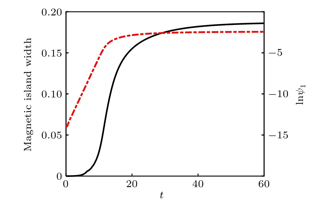
Fig.9. Growth of magnetic island width(the black line)and perturbation of magnetic flux(the red dash line).

Fig.10. Saturated magnetic islands.
5. Conclusion
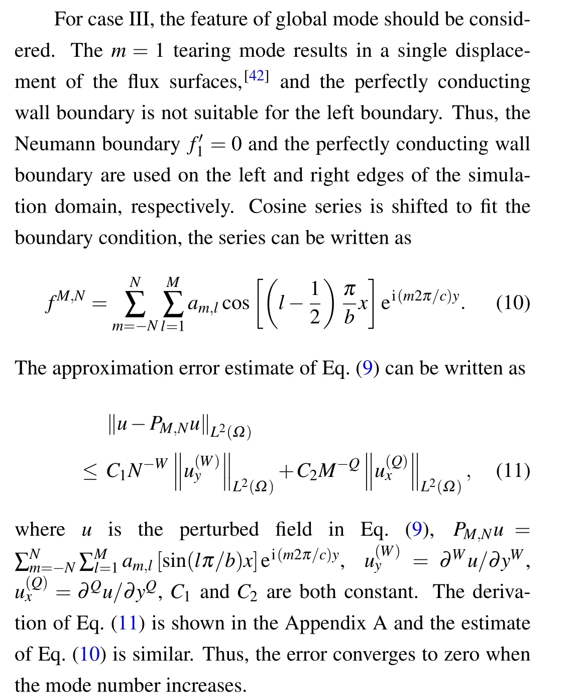
A Galerkin spectral code is developed to simulate tearing modes, which is based on a 2-field RMHD model. Galerkin spectral method is used both in periodic and aperiodic directions. The partial differential equations are solved in the spectrum space,and mode analysis is more convenient in our code.In this paper,both local modes and global modes are simulated with proper boundary conditions. The trial functions are chosen to fit the boundary conditions,and the approximation error is estimated.
The linear results of local and global tearing modes, as well as the nonlinear results of local tearing mode, provide a good fit to the theory. As a comparison, the finite difference collocation code which uses spectral methods in periodic directions is developed. The resistivity scaling results of the two codes are both in accordance with the theory. Compared with the finite difference collocation code,the Galerkin spectral code shows higher accuracy of global modes.The stability analysis demonstrates that the relationship between the maximum time step Δtand the grid numbernis nearly Δt∝n-2when the grid number is sufficiently large. Although the maximum time step of the Galerkin spectral code decreases faster as the grid number increases,still keeps advantages in a range
where the grid number satisfies the convergence condition. In the future work, one will generalize the code to a 3D MHD code of cylindrical geometry or toroidal geometry.
Appendix A: The estimate of approximation error
The Fourier approximation has been discussed in some references.[27,44]The computational domain is (0,π)×(0,2π). DefineSNas the space of the Fourier series, andPN:L2(0,2π)→SNis the orthogonal projection uponSNin the inner product ofL2(0,2π):


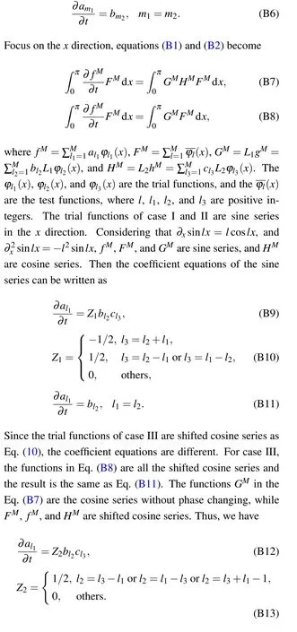
The coefficient equations can be composed of the above equations.
Acknowledgments
Project supported by the Sichuan Science and Technology Program (Grant No. 22YYJC1286), the China National Magnetic Confinement Fusion Science Program(Grant No.2013GB112005),and the National Natural Science Foundation of China(Grant Nos.12075048 and 11925501).
猜你喜欢
小猕猴智力画刊(2021年8期)2021-08-27
阅读与作文(小学高年级版)(2020年11期)2020-12-23
阅读与作文(小学低年级版)(2019年4期)2019-04-20
长江丛刊(2018年6期)2018-11-14
作文评点报·作文素材初中版(2017年42期)2017-11-16
作文评点报·作文素材初中版(2017年42期)2017-11-16
小学生导刊(低年级)(2017年2期)2017-06-10
作文周刊·小学五年级版(2009年6期)2009-04-10
百家讲坛(2008年9期)2008-06-12
军事文摘(2001年11期)2001-10-28

- Chinese Physics B的其它文章
- A design of resonant cavity with an improved coupling-adjusting mechanism for the W-band EPR spectrometer
- Photoreflectance system based on vacuum ultraviolet laser at 177.3 nm
- Topological photonic states in gyromagnetic photonic crystals:Physics,properties,and applications
- Structure of continuous matrix product operator for transverse field Ising model: An analytic and numerical study
- Riemann–Hilbert approach and N double-pole solutions for a nonlinear Schr¨odinger-type equation
- Diffusion dynamics in branched spherical structure