
A spintronic memristive circuit on the optimized RBF-MLP neural network
2022-11-21 09:35YuanGe葛源JieLi李杰WenwuJiang蒋文武LidanWang王丽丹andShukaiDuan段书凯
Chinese Physics B 2022年11期
Yuan Ge(葛源) Jie Li(李杰) Wenwu Jiang(蒋文武) Lidan Wang(王丽丹) and Shukai Duan(段书凯)
1School of Artificial Intelligence,Southwest University,Chongqing 400715,China
2Chongqing Brain Science Collaborative Innovation Center,Chongqing 400715,China
3Brain-inspired Computing and Intelligent Control of Chongqing Key Laboratory,Chongqing 400715,China
4National&Local Joint Engineering Laboratory of Intelligent Transmission and Control Technology,Chongqing 400715,China
A radial basis function network(RBF)has excellent generalization ability and approximation accuracy when its parameters are set appropriately. However,when relying only on traditional methods,it is difficult to obtain optimal network parameters and construct a stable model as well.In view of this,a novel radial basis neural network(RBF-MLP)is proposed in this article. By connecting two networks to work cooperatively,the RBF’s parameters can be adjusted adaptively by the structure of the multi-layer perceptron (MLP) to realize the effect of the backpropagation updating error. Furthermore, a genetic algorithm is used to optimize the network’s hidden layer to confirm the optimal neurons (basis function) number automatically. In addition, a memristive circuit model is proposed to realize the neural network’s operation based on the characteristics of spin memristors. It is verified that the network can adaptively construct a network model with outstanding robustness and can stably achieve 98.33%accuracy in the processing of the Modified National Institute of Standards and Technology(MNIST)dataset classification task. The experimental results show that the method has considerable application value.
Keywords: radial basis function network(RBF),genetic algorithm spintronic memristor,memristive circuit
1. Introduction
Since the birth of the concept of ANN in the 1940s, it has resolved many practical problems that cannot be solved by the human brain or even modern computers in the fields of medicine, economics, biology, automatic control, and pattern recognition.[1–3]As one of the most classical network models,the back-propagation(BP)neural network has greatly accelerated the development of ANN.[4,5]However, its disadvantages of slow convergence speed and poor approximation ability make it incapable of high-precision classification tasks.Hence, user should pay attention to the new network with a more reasonable design when dealing with tasks. The radial basis function(RBF)network is a type of network mechanism similar to the BP neural network,and the concept of RBF was introduced by Powell in 1985.[6,7]Compared with the BP neural network,the RBF neural network has the characteristics of simple structure,fast speed and splendid convergence; meanwhile,it also has the capability of global approximation while ensuring the accuracy of approximation.[8,9]The key to establishing an excellent RBF network model is the generation of basis functions,including the determination of the number,centre and width of basis functions. Beyond that, the model can also adjust parameters adaptively according to the types of classified samples.[10–12]Due to the difficulty with network model construction, scholars try to replace thek-means clustering algorithm with other clustering algorithms,which determines the parameters of hidden layers.[13]Spectral clustering is used in the unsupervised learning stage to complete the optimization of hidden layer parameters.[14]A fuzzyC-means clustering algorithm was proposed to obtain the parameters directly,[15]while leader-follower clustering was applied to initialize the centres of hidden layers automatically.[16]However, the robustness of the network model based on the improved clustering algorithm is not ideal. In other words, the optimal centre and width parameters obtained by the clustering algorithm cannot be synchronously adjusted with the change in the number of basis functions. In addition,there are ways to simplify network parameters,such as using the pruning method on hidden layer neurons to simplify the network structure directly.[17,18]This paper starts with the idea of improving the structure and finding a reasonable method to build up a stable network model.
In recent years,the rapid development of electronic components made it possible to simulate neural networks on circuits, and scholars have carried out a variety of explorations: for example, using a memristor-based multiplication circuit to improve the image processing ability of the cellular neural network (CNN);[19]realizing the ink drop spread(IDS) effect on the neural network by a memristor’s fuzzy logic properties;[20]simulating the weight update progress of synapses by a memristor-bridge to complete the random weight change(RWC)learning algorithm on multi-layer neural networks.[21]Evidently, all of this reasearch should be attributed to the creation of memristors. In 1971, Leon Chua proposed the concept of the memristor, the fourth fundamental circuit element after resistance, capacitance and inductance.[22]Through unremitting efforts, HP Studios implemented memory behaviour on a nanoscale TiO2device model in 2008.[23]Its excellent characteristics give it potential application value in signal processing, artificial neural networks and non-volatile storage, and it has become one of the innovative breakthroughs in new circuits.[24,25]In general,there are two aspects to the improvement of a memristor’s properties, and one relies on the inherent properties of raw materials,such as fabrication using chalcogenide,polymer organic matter and other new types of materials.[26]The other method improving the memristor’s structure to affect internal electron flow rules, including the spin memristor, which is based on the spin characteristics of electrons.[11,26]
Based on the existing research,this paper makes some advances in network structure optimization and proposes a memristive circuit to realize the network mentioned above. The remainder of the article is organized as follows. Section 2 presents the RBF-MLP network structure model and optimization method on the basis of the RBF neural network.The basic principles and operating characteristics of spin memristors are analyzed in Section 3. Section 4 proposes a hardware circuit to simulate the complete operational flow of the RBF-MLP network. Section 5 verifies the performance of the network through analysis of the experimental results and comparison with other networks.Finally,Section 6 provides a summary of the whole article.
2. RBF-MLP network model and optimization
2.1. RBF network mathematical model
The classical RBF network structure consists of three layers: an input layer, a hidden layer and an output layer, as shown in Fig. 1. The hidden layer is composed of a set of radial basis functions,which can be used to map the input vector to the hidden layer nonlinearly rather than through weight connections. In contrast, the mapping from the hidden layer to the output layer is linear,so that the weights of the network can be solved by linear equations. When the network adopts a Gaussian function as the radial basis function,the activation function of the neural network can be expressed as
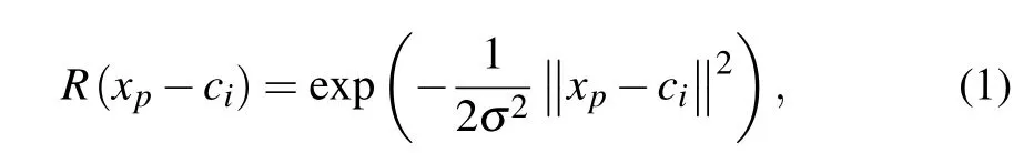
wherex= [xi]Tis the input vector of the neural network,c=[ci]is the coordinate value of the centre point of the Gaussian function when thei-th input vector is used, andσrepresents the width value of the Gaussian function. Assuming that the hidden layer is connected to the weight of the output layerw=[wj],j=1,2,...,n, the output of the radial basis neural network can be expressed as

The critical reason for constructing an RBF network is to determine the parameters of radial basis functions in the hidden layer, including the number of basis functions, centre, variance,weight and other parameters,which are essential factors that affect network capability.[7]If the value of the variance is not big enough,the coverage area of the basis function will be insufficient, affecting the generalization ability of the network. Nevertheless, an excessive value of the variance will reduce the network’s classification accuracy. Therefore, the unsupervised learning process is generally used to obtain the suitable values of the center, variance and the number of basis functions. In thek-means clustering algorithm,hcenters are selected and the local optimal solutionLmaxis obtained through the algorithm;that is,the maximum distance between centres is chosen as the centre of the basis function.[13]By this way, the variances and weights from the hidden layer to the output layer can be expressed as follows:

The output of the radial basis function can be obtained by the relationship of the above parameters. However,k-means local clustering algorithms and other global clustering algorithms are likely to group samples that are close to each other but have different categories grouped into one category;therefore,it is difficult to achieve ideal classification accuracy.This is mainly reflected in the significant disparities in the accuracy results of different sample sets. For some sample sets with relatively regular distribution (the distance between classes is far and the distance within categories is close), the processing results are better and, for those sample sets with irregular distribution (complex interleaving between classes, the distance within classes is far),serious misclassification occurs. Therefore, the performance bottleneck of three-layer RBF mainly comes from the limitations of the clustering algorithm.

Fig.1. RBF neural network structure.

Fig.2. Performance comparison of the MLP and RBF neural network on the Wine data set: (a)10 rounds;(b)30 rounds;(c)60 rounds.
2.2. The RBF-MLP network
The multi-layer perceptron (MLP) is similar to the RBF network in structure, and it is also a feedforward neural network,and includes an input layer,a single or multi-layer hidden layer, and an output layer.[27]The error is calculated using forward propagation, and then supervised learning is carried out using the back-propagation algorithm until the error is lower than the established standard, to achieve better classification ability. A Sigmoid function is used as an activation function in the hidden layer,and the Softmax function is used to map classification results in the output layer.Figure 2 shows the training and test results of the RBF network and MLP for the Wine data set, respectively. In few experimental rounds,the difference in classification ability between the two is not apparent.[28]With the increasing of experimental rounds, the ability gap between the two networks becomes more intuitive.After removing some“bad”results,it can be seen that the performance results of the two networks show an irregular curve with stable upper and lower bounds, and it is evident that the accuracy of the MLP is better than that of the RBF network in both training and testing stages. Although the MLP has the disadvantages of long training time and poor coverage,its better performance provides new ideas for improving the RBF network structure.[29]
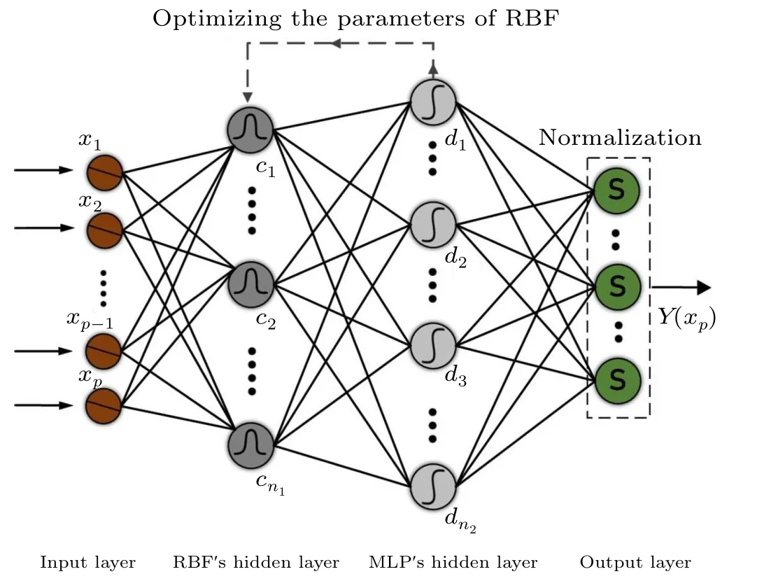
Fig.3. RBF-MLP neural network structure.
Therefore, the operation of the error reverse update can be divided into another more precise part. As shown in Fig.3,the base function of the RBF network’s hidden layer connects to the hidden layer of the MLP through weights for further processing. The error is automatically corrected through the back-propagation of the MLP, and the optimization parameters are sent back to the base function. In the final step, the results are normalized by the Softmax activation function in the output layer.[30]The adaptive error adjustment process of the network shows that, considering the input as the joint action of vectorv, then the inputxpcan be represented by the componentxp(v). The center and variance are initialized asμn(v) andσn(v). The actual outputg(n1)of each basis function is calculated as follows:

Here,srepresents the Sigmoid activation function in the MLP,which is used to map the errors of the hidden layer and make classification judgments;Sis the Softmax activation function that is applied to normalize the probability distribution of the output layer.[30]Under the cooperation of two hidden layers,the basis function could adjust parameters adaptively according to the error value,thus making the complex nonlinear example linearly separable. Compared with the network structure with an external algorithm framework for parameter adjustment,this method of error back-propagation and optimization within the network not only provides more timely error feedback,but also improves the accuracy of parameter adjustment. Furthermore, it avoids the misclassification and multiclassification caused by poor parameter selection to a large extent.
2.3. Automatic parameter searching by using the genetic algorithm.
While optimizing the basis function parameters, the determination of the hidden layer scale is equally significant,i.e.,the valuen1,n2in the RBF-MLP structure affects the performance of the network as well. To be widely applicable to all kinds of sample sets, it is necessary to increasen1andn2as much as possible to reduce the amount of data processed by each unit. In this case, although the classification effect is guaranteed, it will lead to a series of generalization errors,such as the phenomenon of overfitting. In addition to this,the scale of the network will become uncontrollable with the increase in the sample set. Therefore, the values ofn1andn2must be elastic and adaptive.
A genetic algorithm (GA), also known as an evolutionary algorithm, is a search algorithm based on Darwin’s theory of evolution.[31,32]The specific concept is: assuming the problems to be solved are the process of biological evolution;eliminate the solutions that do not adapt to the task through a series of processes,such as crossover,mutation and evolution;retain the highly adaptable solutions in the later generation and repeatedly evolve;and finally obtain the optimal solution by decoding the optimal individuals in the last generation.[33]Therefore,in this paper,obtaining the optimal network structure can be considered as a task requiring constant evolution,and the optimaln1andn2values can be regarded as the optimal solution to the problem. The overall operation process is shown in Fig.4.
The first step is population initialization,which is related to whether the whole genetic algorithm can finally converge to the global optimal solution. For the small-scale optimization problem in this paper, the random number generation method is used. Then, the fitness function is called for calculation,and the fitness obtained determines whether it is the optimal solution or not.[34]If not,we then select the best contemporary individual to proceed with subsequent operations.To ensure the excellence of the next generation, the binary tournament selection method can be used in the experiment to iterate according to the fitness value and to select the outperformers in the next generation population set.[35]The next step is crossover and mutation, which is also the core of the genetic algorithm and is used to complete genetic operation.Crossover operation refers to the process in which the genes of chromosomes are crossed and part of their chromosomes are exchanged with a certain probability to pass the good genes of the previous generation to the next generation. In this paper,simulated binary(SBX)crossover is adopted: a pair of parent chromosomes represented by seven-bit binary are truncated with the generated random number and recombined to form a new offspring’s chromosome.[36]By generating all the random numbers within the range to solve the binary values, we can generate the distribution coefficientβ, which represents the crossover relationship between the parent generation and the child generation. Then,it can be fitted using the probability density functionC(x),
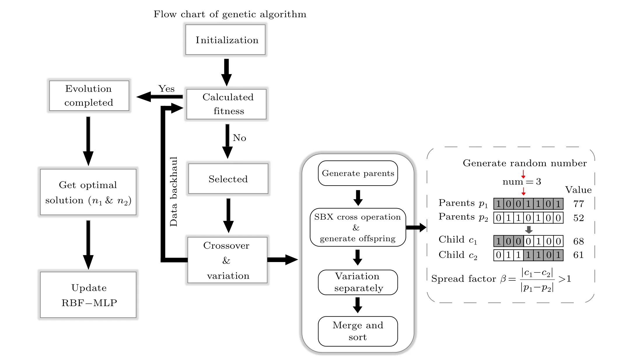
Fig.4. A flow chart of optimization of the RBF-MLP network using the genetic algorithm.

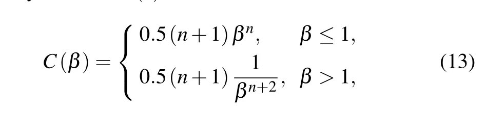
wherenstands for the distribution index and, the largernis,the closer the relationship between the two generations. The distribution function is calculated by the probability density and converted into the cumulative distribution function that is shown in Eqs.(14)and(15),respectively:

The distribution function can represent the crossover situation of each generation intuitively, and the information of the offspring can be obtained through it. After the crossover operation,the set containing the new generation of individuals will have a probability of genetic variation according to the set parameters.To speed up the efficiency of mutation,a polynomial mutation operator is used in this paper.[33,37]The order of decision variables was determined according to fitness, and the individuals corresponding to decision variables were mutated according to the polynomial mutation mechanism.

wherehis a random number within[0,1];nmis the polynomial mutation index;vpis the parent solution; andvl/vurepresent the lower/upper bound of the solution variable. The mutation operator can be expressed as

The early stage of mutation can be regarded as a global search,so the mutation probability is at a relatively high level. As the iteration progresses, the mutation probability will drop to a shallow level;therefore,the mutation probability has an adaptive dynamic change process from high to low, accelerating the convergence to the optimal solution in the later stage of operation. After a series of operations, the new generation is sent back to the fitness function for calculation and judgment.This cycle is repeated until the optimal solution of the problem is obtained: that is, the values ofn1andn2in the RBF-MLP network. Obviously, this method of obtaining parameters using genetic algorithm evolution and an elimination mechanism can be effectively used to determine the optimal network parameters.
3. Characteristic analysis of the spin memristor and crossbar array
3.1. Model of the spintronic memristor
The spintronic memristor is a layered domain wall memristor based on the spin properties of electrons. As shown in Fig. 5, the device consists of two magnetic layers and a thin oxide layer sandwiched between them,one of which is a free magnetic layer with movable domain walls that divide the layer into two magnetically opposite parts.The other layer is a fixed magnetic layer with a fixed magnetization intensity,and its fixed magnetization direction also makes it a reference.[38]When an external current is applied,the position of the domain walls shifts and the resistance changes.The resistance of those parts of the domain that are magnetized parallel to the fixed layer decreases,and that of the other parts increases. According to these properties, it can be seen that the spin memristor has a threshold value. When the domain wall moves to the edge parallel to the fixed layer due to the current action, the resistance value reaches the minimumRoff. When the domain walls move to the opposite parallel edges of the fixed layer,the resistance reaches its maximum valueRon. Because of the nanometer thickness of the domain walls, it is negligible.[11]The resistanceMof the spin memristor can be expressed by
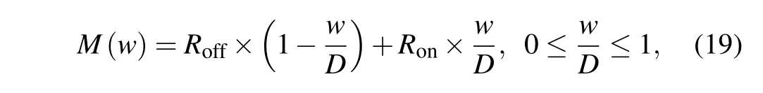
whereWis the width of the part of the free layer that is magnetically parallel to the fixed layer, andDis the total width of the spin memristor. The domain wall velocityvcan be expressed as
whereΓis the domain wall coefficient that is dependent on the material and device structure, which is constant when the material and structure are fixed.Jis the current density,andSis the area of the spin memristor profile. Therefore,the resistance value of the spin memristor can also be expressed as

According to Eq. (20), it can be seen that the domain wall velocityvis proportional to the current density,and the movement of the domain wall depends on whether the current densityJreaches the critical current density or not. When it is greater than or equal to the critical current density, the resistance state of the spin memristor is variable, otherwise it remains constant.
Thus,the resistance of the spin memristor varies with the location of the domain walls, and whether the domain walls change or not depends on whether the current density reaches a critical value. The causal relationship allows the spin memristor to have a stable threshold and to switch characteristics.Compared with conventional memristors, the writing operation in a spintronic memristor is achieved by applying a current through the magnet itself rather than generating a solid reversal field;it is advantageous for a spintronic memristor to offer lower power consumption. In addition, the structure of the spin memristor does not require additional metal wires as current paths,which dramatically improves its scalability.

Fig. 5. (a) The internal structure of the spin memristor. (b) The equivalent circuit of the spin memristor.
3.2. Characteristic analysis of the spin memristor
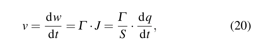
To better illustrate the advantages of this device,this section analyzes the characteristics of the spin memristor utilizing numerical simulation. Firstly,we set the parameters in the circuit as follows:Ron=6 kΩ,Roff=5 kΩ,Γ=1·357×10-11,J=5×10⁷A/cm2,D=1000 nm,s=70 nm2.The input sinusoidal voltage isV=V0sin(2π ft), and the input voltage parameters range from[0.38 1.2]V to[10 50]MHz. Figure 6(a)shows the variation curves of three sinusoidal signals over time. The voltage parameters used in this paper areVa[0.81 V 10 MHz],Vb[0.5 V 10 MHz], andVc[0.42 V 50 MHz], respectively. In Fig.6(b),theI–Vcurves of the spin memristor are the same as those of the model of the memristor in the HP laboratory, showing typical hysteresis loops, which also indicates that the spin memristor continues the excellent circuit characteristics of the memristor. It is worth noting that the hysteresis loop is slightly rough at both ends due to the boundary of the spin memristor, because the resistance is at its maximum at both ends and the voltage and current have a transient linear relationship. Figures 6(c) and 6(d) are the relationship curves between resistance and time or voltage,respectively. Under the applied three sinusoidal voltages, the domain walls move in the free layer from the edge of the same magnetization direction as the fixed layer,so that the resistance changes periodically with the voltage starting from the minimum value ofRoff=5 kΩ. And theM–TandM–Vresponse curves show a horizontal state in a certain period,regardless of the voltage parameters,which means that there is more or less stagnation time for the change in the spin memory resistance value. Obviously,the stagnation is not caused by reaching the maximum resistanceRon. The primary reason for this is that the current densityJcannot reach the critical current density;therefore,the spin memory resistance stops changing the value because of the boundary effect,and the memory resistance remains constant for a period of time until the current density is greater than the critical current density.
It can be clearly seen that the spin memristor device has a pronounced boundary effect and threshold properties,which is different from the threshold properties displayed by the traditional memristor only when the threshold value is at the critical importance.In the HP memristor,the resistance value depends only on the doping concentration of oxygen ions,and does not change its original properties according to the current density.This means the resistance of the memristor can be limited to a constant value betweenRonandRoffby changing the current parameters. Furthermore, it could be effectively applied to circuits to realize a neural network, which contains a large number of weight parameter storage,updates and calculation.
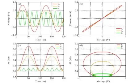
Fig. 6. Circuit characteristic curves of the spin memristor with sinusoidal voltage input of different parameters. (a) Input voltage curve. (b) I–V curve. (c)M–T curve. (d)M–V curve.
3.3. Spin memristor crossbar array
Figure 7 shows a 5×5 cross array of a spin memristor,whose array size can be adjusted according to actual requirements. The resistance value of each node has a bidirectional relationship with the voltage applied in the vertical and horizontal approaches.[25]The resistance value can be changed not only by changing the voltage in the two directions,but also by reading the voltage in the two directions.[24,39]
These contact each other and,independently of the mesh nodes structure, coincide with each other between neurons in a neural network topology structure similar to. Firstly, it essentially provides the ability to combine input signals in a weighted manner,mimicking the dendrite potential.Secondly,according to the characteristics of the synaptic network,it can support a large number of signal connections within a small memory footprint. Therefore, the weight variable of the neural network can change with the change of the resistance of each spin memristor. Moreover, the circuit composed of the memristor cross array can save the model and parameters after training in the case of a power failure. This can avoid repeated parameter optimization when the neural network is used for calculation again,and thus significantly improve the efficiency in practical application.
Fig.7. The spin memristor crossbar array structure.
4. Spintronic memristor-based RBF-MLP neural network design
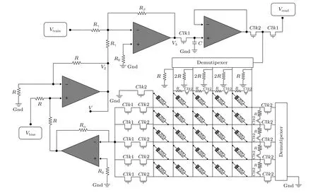
Fig.8. A spin memristor cross array circuit for implementing RBF-MLP networks.
As mentioned above,the spin memristor can be applied to realize neural network functions due to its characteristics such as threshold,non-volatility,low power consumption and high efficiency. The two hidden layers in the RBF-MLP network have different effects; therefore, the overall hardware circuit structure is divided into two parts.The first part is used to simulate the parameter updating operation in the RBF layer,which consists of a 5×5 spin memristor cross array,two demodulators and several NMOS switches for control. The other part is mainly composed of four reverse amplifiers in the peripheral circuit,which is responsible for simulating the MLP layer optimization parameters and error correction.Vreadconverts the read signal between digital and analogue signals through the demodulator; then, the converted signal is input into the cross array circuit. Due to the spintronic memristors’boundary properties, the current density in each direction is controlled to determine whether we need to activate each unit of the cross array.When the two switches on the left are activated simultaneously,the resistance value is converted into a signal and connected to the first reverse amplifier,which is then connected to the peripheral circuit for processing and calculation.Under the effect of the error signalVbiasand the training signalVtrainimposed by the outside successively, the processed signal is returned to the demodulator and compared with the set standard to determine whether to suspend the error updating process or not. The overall circuit structure is shown in Fig.8.
During the circuit operation,each memristor value is initialized betweenRonandRoff.Meanwhile,the memristor cross array can be regarded as an entire resistanceRMfor convenience. To read the whole resistanceRMin the training stage,the NMOS switch is opened under the joint action ofClk1 andClk2,and it is connected to the external circuit as the input of the first-level amplifier. According to the working nature of the invert amplifier,the outputv1of the invert amplifier can be expressed as

Under the influence of input error signals,the outputv2,which is affected byvbias,can be expressed as

The third stage amplifier is responsible for the input of the training signal. To update the value of the memristor array,the ratio ofRβtoRγcan be quantified and set as the training coefficientη:

Based on the above relationship,it can be seen that the value ofv3is not only affected by the joint action of thevread,vtrain,andvbiassignals,but it can also be influenced by the training coefficientη.The weight reading/updating of the neural network can be simulated by three voltage signals,and the training coefficientηis similar to the learning rate,which represents the speed of adjusting the network’s weight by the loss gradient.After error adjustment and training operations, the signalsv3are stored in the capacitorCand released whenClk2 is activated. This switch setting can effectively avoid the disorderly superposition of signals. The signals through this series of operations are sent back to the outside of the demodulator for conversion and comparison with the set parameters. If the comparison results are not ideal, the next round of learning and training operation is re-entered.
It can be seen that this kind of spintronic memristor-based circuit with low energy consumption and small volume can intuitively simulate the running process of the RBF-MLP network. In contrast to other devices,the memristor’s nonlinearity can adjust the value according to the input signal, and the threshold properties of spintronic memristor devices also help to stabilize the circuit parameters. In addition, the resistance value is no longer limited to the rigid boundariesRonandRoff,and this allows the circuit to change parameters by adjusting the current density,which further achieves the effect of adaptively changing the circuit parameters for the updated circuit signal.
5. Analysis of experimental results
In the experimental stage, as the network classification performance test samples must have complexity and diversity,and for comparative experiment,we also take into account the universality of the sample set. In this article, the Modified National Institute of Standards and Technology(MNIST)was chosen as the experimental database, which contains 60000 training images and 10000 testing images,as shown in Fig.9.Meanwhile, to verify the performance of the RBF-MLP network in task classification, the control variable method was used in the experiment to make a horizontal comparison of the specific implementation of the network: according to the characteristics of the network structure, three similar but not completely consistent network models are established. The specific models are shown as follows.

Fig.9. Several examples from the MNIST dataset.
(i)RBF network(hiddenlayer nodes optimized by GA)
The network only contains an RBF neural network, and the genetic algorithm automatically finds the optimal node parameters of the RBF’s hidden layer.The number of basis functions can be determined adaptively,but without adaptive error adjustment.
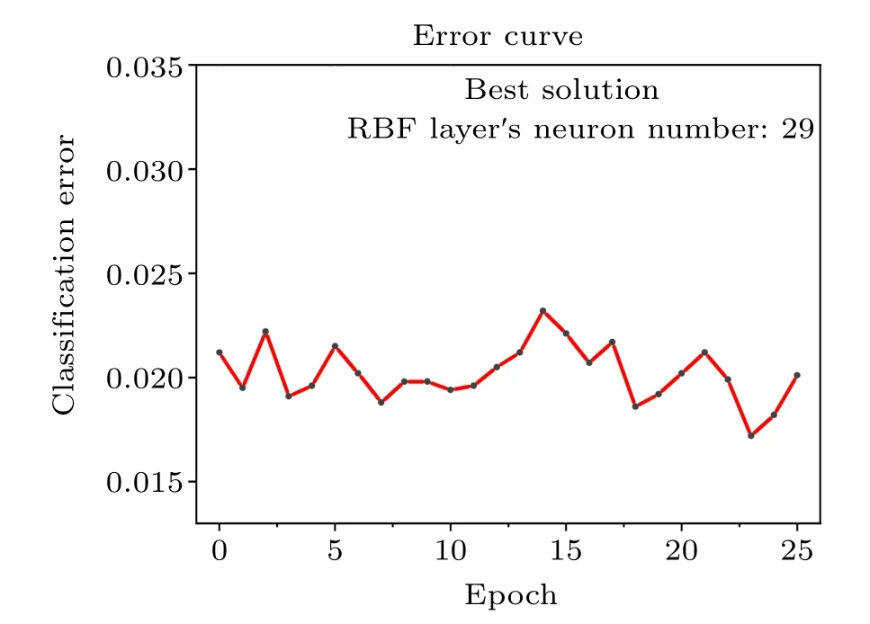
Fig.10. The training error rate curve of the network model(i).
The experimental results are shown in Fig.10. It can be seen that after 25 epochs,the classification error rate remained stable at 0.02.
(ii)RBF-MLP network(only RBF hiddenlayer nodes are optimized by GA)
This model uses a complete RBF-MLP neural network structure. But only the genetic algorithm is considered to optimize the RBF’s hidden layer so that the number of MLP nodes cannot be adjusted automatically. According to the experimental results, the classification error rate decreased with the increase of epochs,and stabilized at 0.175 after 25 epochs,as shown in Fig.11.
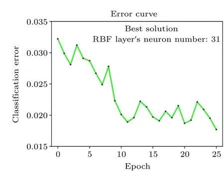
Fig.11. The training error rate curve of the network model(ii).
(iii)RBF-MLP network(RBF&MLP hiddenlayer nodes are optimized by GA)
This model is also an RBF-MLP network structure, but the genetic algorithm is used to optimize the parameters of two inner hidden layers. Therefore, the network’s structure could continuously be improving with the iteration of the genetic algorithm. In Fig.12,we find that the error rate of this structure is the lowest,which can be stable at 0.167. In other words,the classification accuracy rate of the network can reach 98.33%.
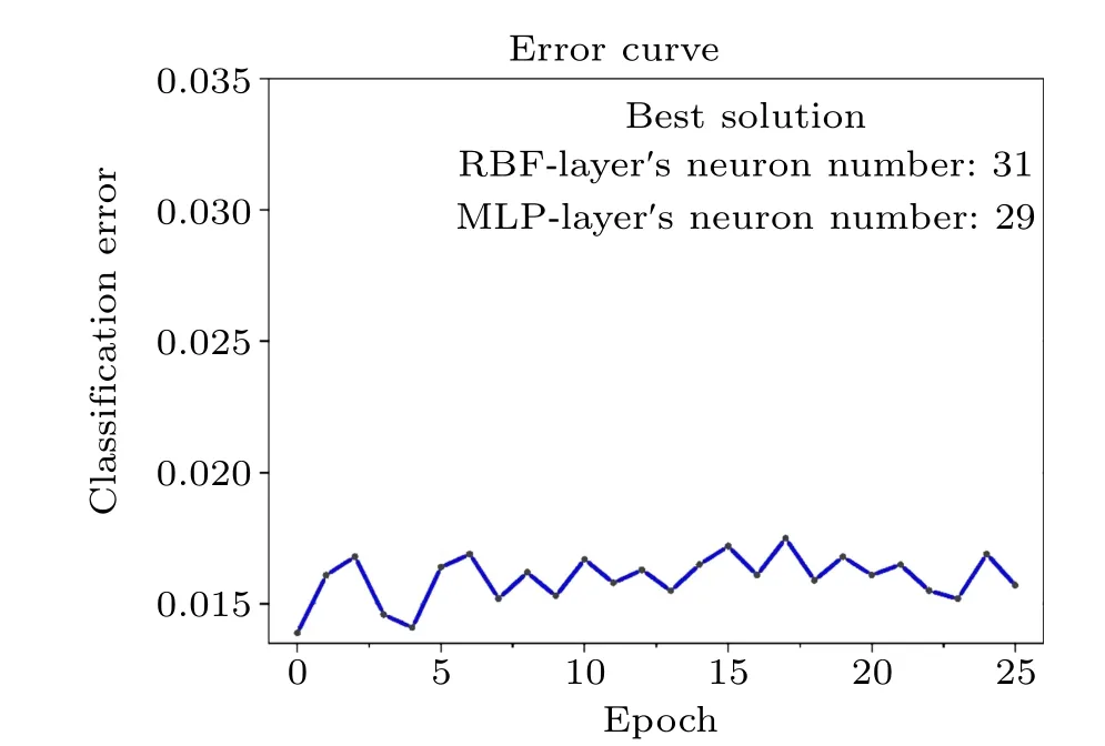
Fig.12. The training error rate curve of the network model(iii).
Based on multiple experiments, the time error of each of 25 epochs under the same operating environment is within 5% (this result will decrease with the functional of the operating environment configuration, such as when using a highperformance graphics card or directly running on the server with high computing power), so there is a minimal gap in efficiency. Therefore,the experimental results not only indicate that the performance of the network can be greatly improved by the genetic algorithm for automatic network search and parameter settings,but also confirm that the performance of the RBF-MLP structure is improved for a single RBF network.In addition, it is worth mentioning that even if the centre and width of the RBF network are randomly initialized, the same precision can be achieved after training,which means that the network model has outstanding robustness.
Table 1 and Figure 13 respectively show the results comparison among various types of RBF neural networks. Obviously, the classification performance of the RBF-MLP is excellent when the algorithm/structure optimization is carried out simultaneously. It is worth mentioning that the accuracy of the FL-RBF-CNN network, which has the best classification effect,increases with the times of the training epochs.[40]By contrast, the RBF-MLP network can maintain relatively stable accuracy from the initial training.This is due to the universality of the best model obtained by the genetic algorithm,which is lacking in other networks.

Table 1. The performances of various optimized RBF/MLP networks on MNIST datasets within 25 epochs.

Fig. 13. Performance comparison of other types of RBF network models on the MNIST dataset. I: The RBF-MLP model optimized by GA. II: The deep-RBF model with gfirst-class loss function.[41] III:The fuzzy logic(FL)RBF-CNN model.[40]
The RBF-MLP network also has outstanding advantages over other types of networks. Figure 14 shows the MNIST training accuracy of the unsupervised spiking neural network(SNN) network based on the spike timing dependent plasticity(STDP)learning rule.[44]As the number of reference vector neurons increases (400–1600–3600–6400), the portion of the input space per neuron decreases, improving accuracy by allowing each individual neuron to be more restrictive in its angular scope. As shown in Table 2, an SNN-STDP with considerable accuracy should contain enough neurons due to its fully-connected one-layer structure,and the RBF-MLP requires a much lower number of neurons to accomplish the same task. Even when the number of neurons reached 6400,the accuracy of the two training tasks remained at the same level.

Table 2.Training accuracy results comparison of the RBF-MLP network and the SNN-STDP network on the Mnist dateset within 25 epochs. Highlighted cells are the best confgiuration for each size.

Fig.14. Performance comparison of the RBF-MLP and the SNN-STDP on the MNIST dataset.
However,after a series of experiments,it is found that the deficiency of the network structure is that it takes a long time in the training phase. It does not matter if the genetic algorithm is optimized or not, such as the training time of the model(b)and(c)length error is 2.4%–3.5%). This is mainly due to the mutation rates of the genetic algorithm and the descending trend with the number of iterations. In the later stages of evolution,extremely low mutation rates lead to an excessively long training time;therefore,obtaining the optimal solution is at the cost of sacrificing efficiency.
6. Conclusion
In this article, we first proposed the RBF-MLP structure according to the bottleneck of the RBF neural network. The centre and width of the hidden layer can be adjusted adaptively by working cooperatively, which solves the problem of confriming the parameters of the basis function. In addition, a genetic algorithm is used to optimize the hidden layer and realize the automatic search of network model parameters.Then,according to the characteristics of the network structure,a spintronic memristor-based circuit is used to simulate the operation of error backpropagation updating and training in the network by combining the memristor device with the external circuit,and a small neural network is realized on the memristor circuit.
The experimental results show that the improved network structure can improve the classifciation accuracy to a certain extent, and the compatibility between the model and the data set can also be improved by invoking the external framework modelling method. In the process of testing with the MNIST data set,the accuracy of classifciation can reach 98.33%when the training amount is constant.However,without considering the improvement of the operating environment confgiuration(such as high-computing-power server or high-performance GPU for processing),the shortcomings of its training duration make further improvement possible,such as adjusting the activation function by further improving the generalization ability and adjusting the mutation rate adaptively according to network feedback. All these points can be used as the directions for further research work.
猜你喜欢
小小说月刊·下半月(2022年7期)2022-07-19
小小说月刊(2022年14期)2022-07-18
客联(2022年3期)2022-05-31
源流(2021年11期)2021-03-25
小天使·一年级语数英综合(2020年3期)2020-12-16
小天使·一年级语数英综合(2020年2期)2020-02-04
新高考·高二数学(2016年7期)2017-01-23
大作文(2015年12期)2015-12-31
短篇小说(2014年11期)2014-02-27
故事林(2010年6期)2010-05-14

- Chinese Physics B的其它文章
- A design of resonant cavity with an improved coupling-adjusting mechanism for the W-band EPR spectrometer
- Photoreflectance system based on vacuum ultraviolet laser at 177.3 nm
- Topological photonic states in gyromagnetic photonic crystals:Physics,properties,and applications
- Structure of continuous matrix product operator for transverse field Ising model: An analytic and numerical study
- Riemann–Hilbert approach and N double-pole solutions for a nonlinear Schr¨odinger-type equation
- Diffusion dynamics in branched spherical structure