
RNAGCN:RNA tertiary structure assessment with a graph convolutional network
2022-11-21 09:32ChengweiDeng邓成伟YunxinTang唐蕴芯JianZhang张建
Chinese Physics B 2022年11期
Chengwei Deng(邓成伟) Yunxin Tang(唐蕴芯) Jian Zhang(张建)
Wenfei Li(李文飞)1,2, Jun Wang(王骏)1,2, and Wei Wang(王炜)1,2,‡
1Collaborative Innovation Center of Advanced Microstructures,School of Physics,Nanjing University,Nanjing 210008,China
2Institute for Brain Sciences,Nanjing University,Nanjing 210008,China
RNAs play crucial and versatile roles in cellular biochemical reactions.Since experimental approaches of determining their three-dimensional (3D) structures are costly and less efficient, it is greatly advantageous to develop computational methods to predict RNA 3D structures. For these methods, designing a model or scoring function for structure quality assessment is an essential step but this step poses challenges. In this study, we designed and trained a deep learning model to tackle this problem. The model was based on a graph convolutional network(GCN)and named RNAGCN.The model provided a natural way of representing RNA structures, avoided complex algorithms to preserve atomic rotational equivalence,and was capable of extracting features automatically out of structural patterns. Testing results on two datasets convincingly demonstrated that RNAGCN performs similarly to or better than four leading scoring functions.Our approach provides an alternative way of RNA tertiary structure assessment and may facilitate RNA structure predictions. RNAGCN can be downloaded from https://gitee.com/dcw-RNAGCN/rnagcn.
Keywords: RNA structure predictions, scoring function, graph convolutional network, deep learning, RNApuzzles
1. Introduction
RNAs play crucial and versatile roles in cellular biochemical reactions, such as encoding, decoding, catalysis,[1]gene regulations,[2]and others. These functions are closely related to the three-dimensional (3D) structures of the RNAs.To determine RNA 3D structure, experimental technics, including cryo-electron microscopy, x-ray crystallography, and nuclear magnetic resonance (NMR) spectroscopy are usually employed. Since these technics are costly and inefficient,computational methods have been developed to predict RNA structures.[3–19]Computational algorithms usually include two steps: (i) generating structural candidates and (ii) selecting structures most likely to be the native. The second step requires a good scoring function that can assess the quality of the candidates.
Traditional scoring functions[20,21]are physics-based or knowledge-based, to name a few, Rosetta,[4,22]3dRNAscore,[23]RASP,[24]RNA KB potential,[25]DFIRERNA,[26]and rsRNASP.[27]Among them, 3dRNAscore is an all-atom statistical potential that combines distance-dependent and dihedral-dependent energies;[23]it is more efficient than other potentials in recognizing and ranking native state from a pool of near-native decoys. The rsRNASP potential is composed of short- and long-ranged energies, distinguished by residue separation along sequence;[27]extensive tests showed that it has higher or comparable performance against other leading potentials, dependent on specific testing datasets. In recent years, machine learning approaches achieved great success in many fields, including computer vision, natural language modelling,[28,29]medical diagnosis,[30]physics,chemistry, computational biology, and so on.[31–34]Inspired by these successes, our group developed a scoring function for the assessment of RNA tertiary structure based on a three-dimensional convolutional network and named it RNA3DCNN.[35]
Applications of graph convolutional network(GCN)[36–41]to represent molecular structures have been quite successful.[42–47]For example, Foutet al.[43]modelled proteins as graphs at residue level and then predicted protein interfaces. Federicoet al.[44]introduced GCNs (GraphQA)to tackle the problem of quality assessment of protein structures, and showed that using only a few features will result in state-of-the-art results. Soumyaet al.[45]developed ProteinGCN for protein structures assessment; they built graphs to model spatial and chemical relations between pairs of atom.Zheet al.[46]built a GCN network, named GraphCPI, which aggregated chemical context of protein sequences and structural information of compounds to tackle the problem of compound–protein interaction. Huanget al.[47]introduced a model called GCLMI based on GCN and an auto-encoder to predict IncRNA–miRNA interactions.
Inspired by the notion that a graph provides a more natural representation of 3D RNA structures and hence may bring better assessing performance, in this study, we upgrade our previous model by changing the convolutional network to a GCN network. Specifically, we developed a network model based on GCN, named RNA graph convolutional network(RNAGCN),to perform quality assessment of RNA structures.We trained and tested the model and compared the results with several leading scoring functions.
2. Materials and methods
In this section,we first introduce the input and output of RNAGCN, and then the architecture of the model. Next, we present the datasets used for training and evaluation,followed by a description of the metrics used to evaluate the performance of the model. At last,we describe the loss function and the training procedures.
2.1. Graph representation of RNA structures
RNA structures can be naturally represented as graphs,with nodes modeling atoms and edges modeling their relative spatial position in three-dimensional space. Since RNA sizes vary, we split an input RNA into many “local environments”and converted each into a graph. Specifically, for theithnucleotide along the sequence, we defined it as the central nucleotide of its “local environment” constructed by including all its nucleotide neighbors. A nucleotide was defined to be a neighbor if any of its heavy atoms (other than a hydrogen atom) was within a threshold spatial distance of any heavy atoms of the central nucleotide. The distance threshold was set to be 14 ˚A.This is to construct a large enough local environment for the central nucleotide.With this design,the model can be scaled to handle RNAs of arbitrary size. Thus, for an RNA of lengthNs,we constructedNslocal environments represented byNsgraphs.
In general,a graph is defined as a set

whereVdenotes the set of nodes andEdenotes the set of edges,respectively.X ∈R|V|×NandU ∈R|ℰ|×Eare the feature matrices ofVandE,respectively.N,Eare the number of nodes and number of edges,respectively.
All heavy (non-hydrogen) atoms in a local environment were treated as nodes. A node was represented as a one-hot vector of lengthNt,whereNtis the total number of atom types,which is 54,based on AMBER99SB force field.
Edges were defined between neighboring atoms. Each atom was connected by an edge with itsKnearest atoms in space, whereKwas set to be 14. Edges were directed and each included five features. The first was the spatial distance betweenSandT, which was one of its neighbors. The 2nd,3rd,and 4th were direction features,which were the three projections of the unit vector pointing fromStoTin the internal coordinate system centered onS,i.e.,
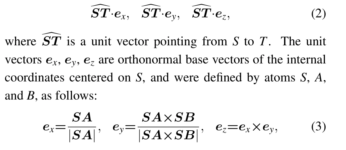
whereAdenotes the ‘C1’ atom andBthe ‘C5’ atom in a nucleotide. The fifth feature had a value of 1 or 0,depending on whether there is a chemical bond betweenSandT.
2.2. Output of RNAGCN:quality score
The graphs representing the local nucleotide environment constructed for each nucleotide from its neighbors were used as input to the GCN model. The model output was a scalar score indicating the quality of the input. During training,the output score measured the difference of local environment from the ground truth, i.e., the RMSD of the input structure with respect to the experimental one. During the inferring operation,the network output was the predicted score indicating the RMSD of the input versus the experimental structure that in this operation was an unknown to the network. The scores thus obtained for theNsinput environments of an RNA were averaged to get the final score,which reflected the overall difference of the input structure to the experimental one, with a lower score corresponding to a higher input quality (a better approximation of the unknown experimental structure).
2.3. Architecture of RNAGCN
RNAGCN is a deep learning model based on GCN that is used to extract features from 3D structures of RNA. The model architecture is shown in Fig. 1. The input to the model is an RNA local graph,converted from an RNA local environment. Below the input layer,there are five serially connected graph convolution layers that operate on the graph sequentially.Residual modules and skip connections were adopted to solve the gradient vanishing problem often seen in deep neural networks.[38,40]Serially connected below the GCN layers,there is a convolution layer with a 1×1 kernel, followed by a graph global max pooling layer, and then the final layer of a fully-connected network that outputs a score as prediction.The model contains about 378k parameters in total.
In the five GCN layers, graph convolution operations were used to update the nodes’representations iteratively. The details of the operations are shown on the right side of Fig.1.

Fig.1. Overview of the RNAGCN model. The input is an RNA local graph. The network contains five graph convolution layers,a convolution layer with a 1×1 kernel,a graph global max pooling layer,and a fully-connected network that outputs a score as prediction. The right panel presents details of feature operations using graph convolution with residual connections.
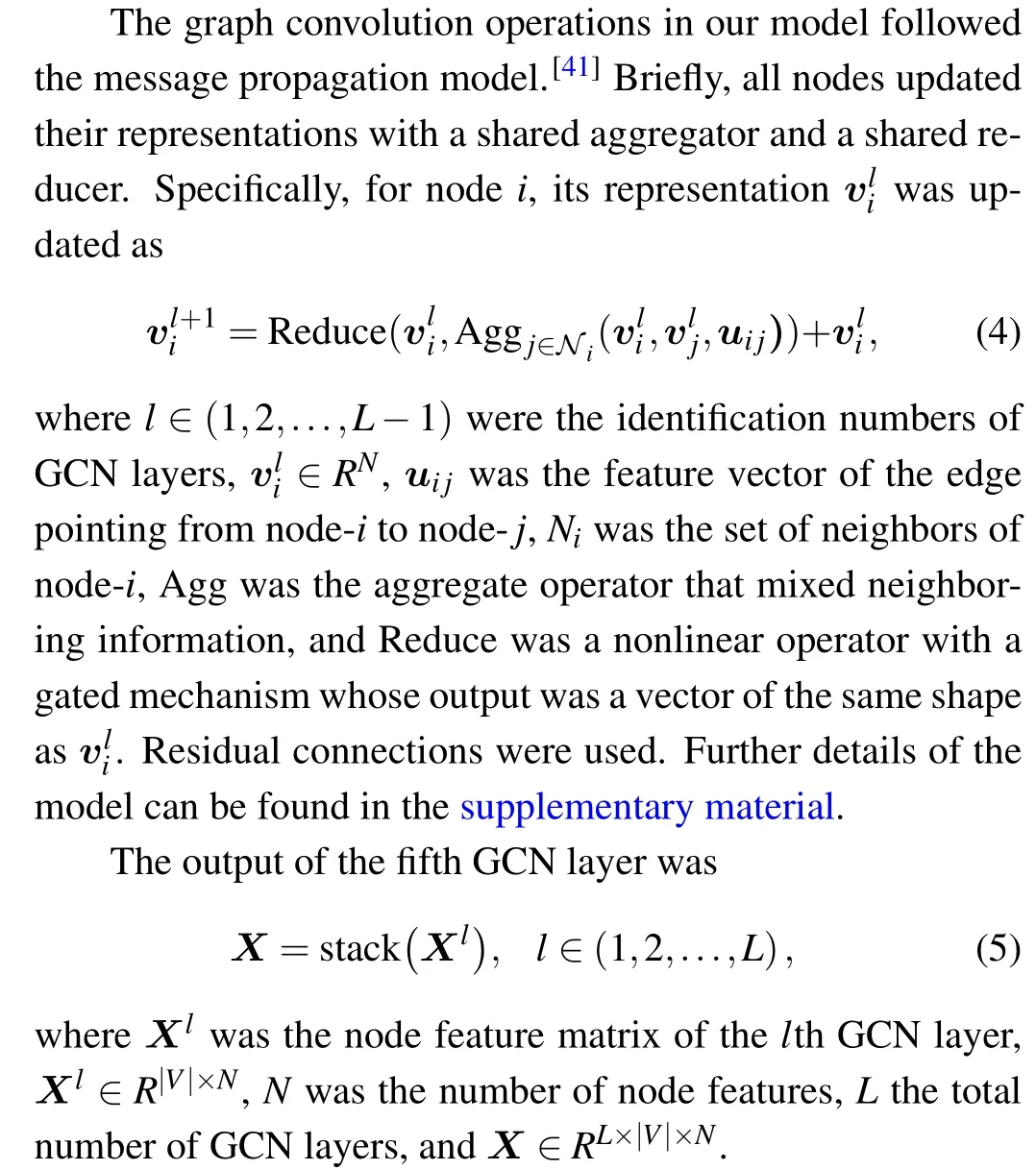
Following the GCN layers, a convolution layer with a 1×1 kernel was used to perform the aggregation of information fromLGCN nodes with different weights. These weights were learned from data during training. As a result,Xwas reduced fromRL×|V|×NtoR|V|×N.
A global max pool layer was used to mix nodes representations. Max values ofX ∈R|V|×Nalong|V|were computed one by one. As a result,Xwas further reduced,fromR|V|×NtoRN.
Finally,a fully-connected network was used to reduceXfromRNtoR1.It included a layer of size 64 with ReLU activation function,and a layer of size 1 without activation function.
Notably, the representation of edges was kept static during graph convolution,according to the generally accepted notion that updating nodes’features alone is usually sufficient to achieve reasonable model performance.
2.4. Datasets
We built our datasets based on the non-redundant set of RNA 3D Hub[48](http://rna.bgsu.edu/rna3dhub/nrlist,Release 3.102, 2019-11-27). RNAs forming complex with proteins or other molecules were removed; only pure RNA structures were kept. Short RNAs with length smaller than eight nucleotides were also removed. The remaining 610 RNAs were split into training, validation and testing datasets. The infernal program[49]was used to ensure that no RNA in the testing dataset belonged to the same RFAM family as in the training and validation datasets. The resulting three datasets contained 426, 92, and 92 RNAs, respectively. Hereafter, the testing dataset of 92 RNAs is referred to as Test-I.
RNA decoys are needed to train and test scoring functions. From the experimental structure of each RNA, we generated the corresponding decoys with high-temperature molecular dynamics (MD) simulations, carried out using Gromacs.[50]In brief, each RNA molecule was solved in a TIP3P water box,and metal ions were added to neutralize the system. The system was then subjected sequentially to energy minimization, NVT equilibration, and NPT equilibration at 300 K.Finally,high temperature MD was used to denature the structure by gradually increasing the temperature from 300 K to 660 K.The force field was AMBER99SB.Each simulation lasted for 10 ns. For each trajectory,we calculated the RMSD of each frame with respect to the corresponding experimental structure and randomly selected 200 decoys in the RMSD range from 0 to 20 ˚A. The decoys, together with all the experimental structures,constructed the training,validation,and testing datasets,as summarized in Table 1.
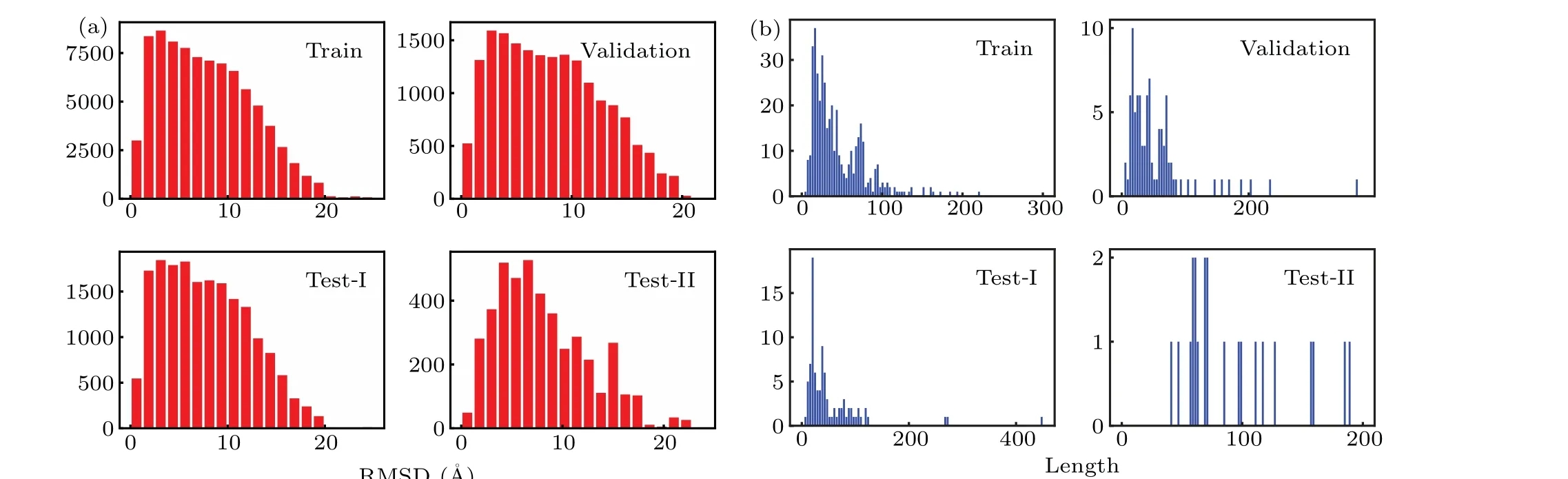
Fig.2. Distributions of(a)RMSD and(b)length for four datasets. Note that RNA 6qkl in the training set is not shown,for its length is too long(1158 nucleotides).
We prepared another testing dataset based on the RNApuzzles-standardized dataset,[51]which included 22 RNAs.Again, for each RNA in this set, the same denaturing procedure was carried out by high-temperature MD to generate decoys, and 200 decoys were randomly selected. The resulting testing dataset,referred to as Test-II hereafter,contained 4422 RNA structures.
The distribution of RMSDs and lengths for the abovementioned datasets are given in Fig.2.

Table 1. Information of datasets.
2.5. Evaluation metrics
Enrichment score (ES) and Pearson correlation coefficient(PCC)were used to evaluate the performance of scoring function.
Enrichment score(ES)[23,25–27,35,52]was defined as

whereStop10%andRtop10%indicated the best-scored 10% decoys and the 10% with the lowest RMSDs, respectively.Ndecoyswas the number of decoys associated with the RNA of concern. ES values ranged from 0 to 10, with larger value indicating better performance.
The Pearson correlation coefficient (PCC)[24,27,52]indicates the magnitude of linear correlation between two variables and is defined as

whereSiandRiare the scores given by the scoring function and the RMSD of the structure, respectively. PCC assumes a value between 0 and 1.
2.6. Loss function
The loss function, used as the optimizing target of the model,was defined as

whereRiandSiwere RMSD and the predicted score of theithlocal environment,respectively.Nenvswas the total number of local environments in the whole training dataset. In this study,it amounts to about 107.
2.7. Training strategies
All the RNAs were partitioned into local environments,which were then randomly shuffled and fed to the network in batches. The batch size per GPU was set to 64 and the total batch size was 384, since 6 GPUs were used in parallel computation. Python modules Deep Graph Library and Pytorch.Distributed were used for model construction and computation parallelization,respectively. Mini-batch gradient descent algorithm was employed to train the model.Specifically,the Adam optimizer with parametersβ1=0.9,β2=0.98 was used. The initial learning rate was 0.004 and it would be decreased by half if the training loss no longer dropped for 4 epochs.
3. Results
In this section,we present the results of our model experiments and compare the performance of our model with four statistical potentials, including RASP, Rosetta, 3dRNAscore,and rsRNASP, which are currently the most popular in the field.
3.1. Performance on Test-I
Table 2 shows the performance of the five models in assessing the quality of structures in the Test-I dataset, which contained 92 RNAs and 200 decoys associated with each.We used two criteria, labeled as Top-1 and Top-5, to reflect whether the experimental RNA was ranked the first,or ranked among the best five, respectively. As judged by Top-1, 3dRNAscore and rsRNASP performed best;they identified 91 and 86 out of 92 RNAs,respectively. RNAGCN(our model)performed as a third (79/92). Judged by the criterion Top-5, all models performed similarly. According to comparisons based on these two criteria, our model is the third best among all.This outcome is tentatively attributed to the strict criteria we used to construct the testing set: we made sure there are no overlapping of RFAM families between the testing set and the training datasets.
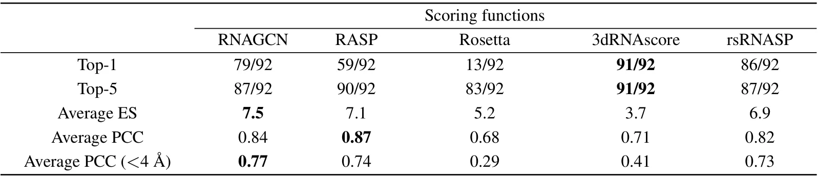
Table 2. Performance of five models on Test-I.

Fig.3.(a)Experimental structure of RNA 5dcv.(b)Score-RMSD plots,showing the correlation between the scores predicted by the model and the RMSDs of the structures. The purple crosses mark the experimental structures, orange crosses indicate the structures that were scored better than the experimental ones, and red crosses mark the best-scored structures if they were not the experimental one.
Table 2 also presents the average values for ES and PCC that indicate the strength of correlations between the ground truth and prediction.Our model is superior to the others by the ES measure, close second best behind RASP by the average PCC, and clearly superior by the measure sensitive to nearnative structures (PCC with RMSD<4 ˚A). The latter result indicates that our model excels at discriminating small structural changes with respected to the native one.
In Fig. 3(b) we present the score-RMSD plots for each of the five models, computed using RNA-5dcvas an example(Fig.3(a)),which is a 95-nucleotid-long fragment fromP.horikoshiiRNase.[53]The data show that RASP and Rosetta failed to identify the experimental structure as the best one.In contrast,3dRNAscore,rsRNASP and our model ranked the experimental one as the best structure(as indicated by overlapping symbols for best score and native). Moreover,our model appeared to show a better score-RMSD correlation, particularly at small RMSD ranges.For a further proof,we calculated the average PCC values for RNAs within the 0 to 4 ˚A range of RMSD and found them to be 0.77,0.47,-0.65,0.61,and 0.70 for RNAGCN, RASP, Rosetta, 3dRNAscore, and rsRNASP,respectively. By this measure, our model clearly exhibited a significantly higher correlation between scores and RMSDs.This result is also consistent with that bottom line in Table 2,which shows that our model gives the best correlation in the small RMSD range. Moreover, for this specific RNA,the ES values of RNAGCN, RASP, Rosetta, 3dRNAscore, and rsRNASP are 5.0,3.0,1.0,0.5,and 5.0,respectively,also consistent with the ES result presented in Table 1.
The ES, PCC, and score-RMSD plots for each RNA in Test-I are listed in the supplementary material.
3.2. Performance on Test-II
We also analyzed the performance of the five models on the Test-II testing dataset, which is composed of 22 RNAs taken from RNA-puzzles-standardized datasets. The result is summarized in Table 3.
Table 3 shows that 3dRNAscore identified all 22 experimental structures correctly and our model identified just one less, 21 out of 22 RNAs, a close second. Judged by the ES values, our model is 6.5, which is very closed to the best 6.7(rsRNASP).The average PCC of our model is 0.88,also very close second to the best value 0.90 (rsRNASP). Within the small RMSD range (<4 ˚A), the PCC value of our model is again close to the best 0.76 (rsRNASP). Detailed results for each RNA in Test-II can be found in the supplementary material.

Table 3. Performance of five models on Test-II.

Fig. 4. (a) Experimental structure of puzzle-2 in the RNA-puzzles dataset. (b) Score-RMSD plots, showing the correlation between the predicted scores and the RMSDs of the structure. The purple, orange,and red crosses are defined in the same way as in Fig.3.
Figure 4(b)shows the score-RMSD plots for puzzle-2 in Test-II.The pattern of performances is similar to that of Test-I in Fig.3. Three models, including 3dRNAscore, rsRNASP,and ours,correctly identified the experimental structure out of decoys. For this specific RNA, the ES value of our model is 9.5,very closed to perfect value 10;and the PCC value is 0.95.Our model and RASP appear to show a good correlation between scores and RMSDs, while Rosetta, 3dRNAscore, and rsRNASP feature a big gap in scores between the experimental structure and the decoys. The score-RMSD plots for other RNAs in Test-II are generally similar to Fig.4 and listed in full in the supplementary material.
We compiled a detailed ranking of the five models for Test-II and presented the results as a colormap in Fig.5. For each RNA in Test-II and each scoring function, we selected the best-scoredNb(a pre-set variable, “b” indicates best) decoys and computed their average RMSD. We then ranked five scoring functions based on these RMSDs and represented the ranks with different colors, with lighter colors indicating higher ranks. It can be seen that RNAGCN has the largest area of light colors(light yellow and gold),indicating that our model gives the lowest RMSDs more often than the others.
Following the usual practice in the field of machine learning,we plotted receiver operating characteristic(ROC)curves on difference choices ofNb, used as a variable threshold to select structures as the best predicted ones. For example, ifNbwas 10, we trusted the best scored 10 structures ranked by the model as the predicted native structures. To test the model performance under different choices ofNb,we first defined a native ensemble as all structures with RMSD smaller than 2 ˚A,and then defined all structures within the native ensemble as positive samples and the others as negative. These structures and the associated binary classification labels were used to construct the ground-truth dataset, following conventions in machine learning field.During predictions,the bestNbstructures given by model were treated as the predicted positives,while the leftover was treated as the predicted negatives.Under varying choices ofNb, we calculated the true-positive rate (TPR) and false-positive rate (FPR) and plotted their relationship as ROC curves in Fig. 6. It can be seen that the ROC curve of our model almost envelopes (i.e., maximizes)the other four curves. Quantitatively, the areas under ROC(AUC) of our model for Test-I and Test-II are 0.97 and 0.89,respectively; both represent the best performance among the all scoring functions.

Fig. 5. Ranking of five models based on the average RMSDs on the best-scored Nb structures, where Nb is a variable plotted on the x-axis.Each row corresponds to one RNA in Test-II(a total of 22,note their labels are not continuous in the standard dataset). The ranks are indicated by the color bar on the right;the lighter the color,the higher the rank.
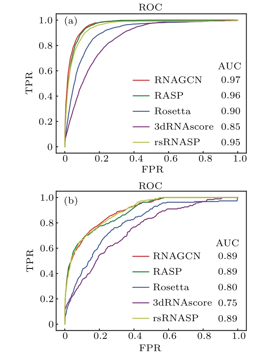
Fig.6. ROC curves of five scoring functions on different choices of threshold Nb. Panels (a) and (b) are results obtained for the datasets Test-I and Test-II,respectively.
4. Discussion and conclusions
Applications of deep learning technology in molecular representation learning have achieved impressive progress in recent years. Inspired by previous works,we explored the application of graph convolutional network in RNA 3D structure assessment tasks. We compiled two datasets with MD simulations and trained a GCN neural network. We tested the model and evaluated its performance using four leading scoring functions. The testing dataset Test-I contained 92 RNAs. Dataset Test-II contained 22 RNAs,a subset of the RNA-puzzles standardized dataset.
For both testing datasets,the ability of our GCN model to identify experimental structures closely approached the best–3dRNAscore on Test-I and rsRNASP on Test-II,respectively.The ES metric,measuring the overlap of the near-native structures and the best scored structures, indicated that our model is the best one for distinguish near-native structures (<4 ˚A)on Test-I while the second one on Test-II. Additionally, we ranked five models based on average RMSD of the best scored structures, and compared their ROC curves and AUCs; both experiments ranked our model as superior to the others.
It is interesting to compare our machine learning model with the statistical potentials based on inverse-Boltzmann equation,particularly,3dRNAscore and rsRNASP.According to the presented results, our model seems to perform slightly worse in identifying native structures (Tables 2 and 3) and slightly better in comparison of AUCs. This outcome may be tentatively attributed to the strict criteria we used to construct the testing set: we made sure there are no overlapping of RFAM families between the testing set and the training datasets. Besides, we did not train the model over and over to increase the metrics,since too much training might lead to over-fitting and then decrease generalization ability, even the training and testing datasets were strictly separated.
In general, the advantages of statistical potentials based on inverse-Boltzmann equation are their clear physical picture,good generalization ability to unseen structures,and fast computation speed. In contrast,machine learning based potentials are black-boxes and have unclear generalization ability and arguably slow speed.However,the advantages of machine learning approaches are also prominent. First,it needs not years of studies looking for proper energy forms and choice of reference states.[52]For RNA structures,it has taken people a dozen years to achieve the current performance. While a similar performance can be achieved by simply taking a general deep network(with slightly modifying the input and output layers)and training it properly. This advantage becomes more prominent if people need to migrate model to new molecules. Second,deep neural networks have found physical patterns similar to those found by human,and have the potential to find new patterns not-known yet. Machine learning based scoring models deserve to be studied.
A recently introduced geometric deep learning approach named ARES[54]showed good performance at scoring RNA structures, but unfortunately, it is not yet possible to directly compare it to ours. The authors of ARES have not released their trained model, and we failed to reproduce their results by attempting to rebuild the model from downloaded codes and training the same network with their datasets. Moreover,ARES was trained on datasets generated with FARFAR2,different from the datasets we generated from MD simulations.A fair comparison of these two models requires identical data or data sampled from independently identical distribution for training and testing.
Our model has several advantages. First, it is natural to represent the geometric and topologic information about RNA tertiary structures as a graph. Second, because a graph automatically provides geometric invariant representation regarding atomic translation and rotation, there is no need to design complex convolution operations such as those used in ARES.Third,because our model can directly learn from spatial patterns of atoms on its own, it requires, unlike physicsbased scoring functions,no prior physical knowledge. Therefore, our approach can be easily extended to other molecular systems with little modification. Forth, the design of splitting structures into local environments makes the model scalable,enabling us to treat RNAs of arbitrary size. At last,this study showed that our model performed well particularly for near-native structures. We tentatively attributed this feature to the graph representation of tertiary structures, for both graph topology and edge features are sensitive to the changes in positions of atoms.
There are two notable limitations of the present work.One limit is computational, stemming from the huge memory consumption of graphs and the massive computations involved in graph convolution operations. As both factors limit the size of the graph,and the number of neighbor atoms around the central nucleotide,they may raise problems handling very long-range interactions that are relevant. The second is algorithmic,as in the current version of the model only node features in the network were updated while edge features were kept static. Presumably,updating both in an upgraded version may slightly improve model performance.
Acknowledgements
This study was funded by the National Natural Science Foundation of China(Grant Nos.11774158 to JZ,11934008 to WW,and 11974173 to WFL).The authors acknowledge High Performance Computing Center of Advanced Microstructures,Nanjing University for the computational support.
- Chinese Physics B的其它文章
- A design of resonant cavity with an improved coupling-adjusting mechanism for the W-band EPR spectrometer
- Photoreflectance system based on vacuum ultraviolet laser at 177.3 nm
- Topological photonic states in gyromagnetic photonic crystals:Physics,properties,and applications
- Structure of continuous matrix product operator for transverse field Ising model: An analytic and numerical study
- Riemann–Hilbert approach and N double-pole solutions for a nonlinear Schr¨odinger-type equation
- Diffusion dynamics in branched spherical structure