
Data-driven Simulations of Magnetic Field Evolution in Active Region 11429:Magneto-frictional Method Using PENCIL CODE
2024-03-22 04:11VemareddyrnWarneckeandPhBourdin
P.Vemareddy , Jörn Warnecke, and Ph.A.Bourdin
1 Indian Institute of Astrophysics, Sarjapur road, II Block, Koramangala, Bengaluru-560 034, India; vemareddy@iiap.res.in
2 Max-Planck-Institut für Sonnensystemforschung, Justus-von-Liebig-Weg 3, D-37077 Göttingen, Germany
3 Institute of Physics, University of Graz, Universitätsplatz 5, A-8010 Graz, Austria
Abstract Coronal magnetic fields evolve quasi-statically over long timescales and dynamically over short timescales.As of now there exist no regular measurements of coronal magnetic fields,and therefore generating the coronal magnetic field evolution using observations of the magnetic field at the photosphere is a fundamental requirement to understanding the origin of transient phenomena from solar active regions(ARs).Using the magneto-friction(MF)approach,we aim to simulate the coronal field evolution in the solar AR 11429.The MF method is implemented in the open source PENCIL CODE along with a driver module to drive the initial field with different boundary conditions prescribed from observed vector magnetic fields at the photosphere.In order to work with vector potential and the observations, we prescribe three types of bottom boundary drivers with varying free-magnetic energy.The MF simulation reproduces the magnetic structure, which better matches the sigmoidal morphology exhibited by Atmospheric Imaging Assembly (AIA) images at the pre-eruptive time.We found that the already sheared field further driven by the sheared magnetic field will maintain and further build the highly sheared coronal magnetic configuration, as seen in AR 11429.Data-driven MF simulation is a viable tool to generate the coronal magnetic field evolution, capturing the formation of the twisted flux rope and its eruption.
Key words: Sun: corona – Sun: evolution – Sun: magnetic fields – Sun: photosphere
1.Introduction
Solar eruptive events like flares and coronal mass ejections(CMEs) are energetic, large-scale phenomena of scientific interest due to their significant impact on space weather.From several studies based on observations and numerical modeling(Klimchuk 2001;Priest&Forbes 2002),it has been established that these large-scale events are magnetically driven by the storage of magnetic energy and helicity in the coronal volume of the active regions (ARs).From this point of view,understanding the structure and evolution of the coronal magnetic field has become an important element in revealing the physical origins of these events on the Sun.
As of now, regular measurements of the magnetic fields are available at the photospheric surface (Scherrer et al.1995;Schou et al.2012) at high resolution and cadence.Continuous vector field observations of magnetic fields from Helioseismic and Magnetic Imager (HMI) onboard the Solar Dynamics Observatory (SDO, Hoeksema et al.2014) had been used in several studies of the magnetic field dynamics, relating their connection to the coronal features present before the occurrence of the flares/CMEs.Since the magnetic fields are line-tied,they become twisted and sheared by the corresponding photospheric plasma motions.These signatures of stored energy magnetic configurations are reported to exist in several ARs exhibiting shearing and rotating motions of the sunspot polarities(Ambastha et al.1993; Brown et al.2003; Tian &Alexander 2006; Vemareddy et al.2012).The configurations with stored magnetic energy are referred to as magnetic nonpotentiality, which was used to quantify in terms of parameters such as the magnetic shear(Hagyard&Rabin 1986;Wang et al.1994),horizontal gradient of longitudinal magnetic field(Falconer et al.2003;Song et al.2006;Vasantharaju et al.2018), electric current (Wang et al.1994; Leka et al.1996),average force-free twist parameter αav(Pevtsov et al.1994;Hagino&Sakurai 2004;Vemareddy et al.2012),magnetic free energy(Metcalf et al.2005),etc.Further,magnetic nonpotentiality was suggested to be linked with sigmoidal-shaped plasma loops in the extreme ultraviolet (EUV) or soft X-ray observations of the corona and are the precursor features(Rust& Kumar 1994, 1996; Canfield et al.2007).Using the continuous vector magnetic field observations, it was possible only recently to show that the coronal accumulation of magnetic energy and helicity is predominant in the ARs exhibiting shearing and rotating motions (Liu & Schuck 2012;Vemareddy 2015, 2019; Dhakal et al.2020) and those ARs produce violent coronal activity.
Since routine observations of the coronal magnetic fields are not available, the photospheric magnetic field measurements are typically extrapolated into the corona to reconstruct the three-dimensional (3D) magnetic structure of the AR corona(Sakurai 1989).The coronal field is approximated as force-free owing to low beta plasma (Wiegelmann & Sakurai 2012) and its evolution is modeled as a series of quasi-static force-free fields.These extrapolated fields are employed to study the coronal magnetic structure containing the null points and flux rope topology (Masson et al.2009; Vemareddy & Wiegelmann 2014; Guo et al.2016; Vemareddy & Demóulin 2018)and are judged to be reproduced structures resembling the observed coronal plasma loops to a high accuracy (Schrijver et al.2008; Vemareddy &Demóulin 2018; Vemareddy 2019).However, the extrapolated magnetic fields represent static fields where the dynamic evolution is missing.Magnetohydrodynamic (MHD) simulations are a viable tool to generate the dynamical evolution of the magnetic fields in the AR corona.These simulations involve advancing the full MHD equations in time and require information about plasma flow,density and temperature in addition to the magnetic field (e.g., Mikić et al.1999; Gudiksen & Nordlund 2002, 2005a, 2005b; Bingert &Peter 2011) in the computational domain.These types of models were very successful in reproducing the magnetic field and loop structure above ARs (Bourdin et al.2013; Warnecke& Peter 2019a).The type of coronal heating in such observationally driven models seems more consistent with MHD turbulence than with the dissipation of Alfvén waves(Bourdin et al.2016).
Although it is physically realistic to capture various processes like flare reconnection, it is computationally expensive to perform on AR scale over a timescale of a few days, even if one enhances the time step significantly(Warnecke&Bingert 2020).As the magnetic field in a coronal model is almost force-free between about 6 and 60 Mm in height (Peter et al.2015; Bourdin et al.2018), alternative methods that may be used to model the coronal field are the ambipolar-diffusion and magneto-frictional (MF) approaches.While ambipolar diffusion would include only a magnetic resistivity parallel to the field B, this method focuses on relaxing an initially known coronal field configuration.We see that this relaxation is sufficient to generate helicity(Bourdin&Brandenburg 2018).The MF approach uses a different resistivity term in the induction equation that depends on the current density J that could still point in any direction.
The MF method (Yang et al.1986) can be utilized to simulate a continuous time series of force-free fields by evolving an initial coronal field by changing the photospheric magnetic field continuously (Mackay et al.2011).In this approach, only the induction equation is used with the assumption that the plasma velocity is proportional to the Lorentz force(Mackay et al.2011)and therefore the initial field relaxes to a force-free field by advancing the magnetic induction equation.The initial field evolves with the corresponding change of the observed lower boundary and preserves the magnetic connectivity and flux from one time instance to the later one smoothly.These simulations have been shown to be effective in capturing comparable coronal field morphologies that resemble each other in EUV images, which are utilized to study the coronal field evolution involving filament channel and flux rope formations (Cheung & DeRosa 2012;Gibb et al.2014; Pomoell et al.2019; Keppens et al.2023).Compared to full MHD, the MF simulations are computationally less expensive and typically much faster; hence, they can be used to study the evolution of coronal fields over long timescales.
In this study, by using the MF approach, we simulate the coronal field evolution in the AR 11429.The method is implemented in PENCIL CODE(Pencil Code Collaboration et al.2021), which is open source and freely available under GitHub.4http://github.com/pencil-codeWe drive the initial field with different boundary conditions (bcs) prescribed from observed vector magnetic fields and then analyze the coronal field evolution over a span of three days.The simulation method and numerical implementation are described in Section 2, the output results of the simulation are presented in Section 3 and a summary and conclusions are given in Section 4.
2.Numerical Simulation
2.1.Magneto-friction Method
The coronal magnetic field evolution of AR 11429 is simulated by the MF relaxation method(Yang et al.1986).It is a special case of the more general MHD relaxation method,which tries to solve the momentum and magnetic induction equations to obtain an equilibrium state.In the MF method,the magnetic field evolves in response to the photospheric foot point motions through the non-ideal induction equation
where vMFis the MF plasma velocity, A is the vector potential relating the magnetic field as B=∇×A and J=∇×B/μ0is the electric current.Solving the induction equation in terms of A ensures that ∇·B=0 is always fulfilled.We choose a magnetic diffusivity of η=2×10⁸m s-2to be able to run the simulation stably.Under the assumption of magneto-static conditions, the momentum balance equation yields the plasma velocity as defined by
where ν is the MF coefficient controlling the speed of the relaxation process and μ0is the magnetic permeability in vacuum.As suggested in Cheung & DeRosa (2012), the frictional coefficient ν cannot be uniform because it will lead to unphysical vMFat the lower boundary,and therefore we used a height-dependent functional form given by
where ν0is set around 80×10-12s m-2,z is the height above the bottom boundary and L is chosen as 15 Mm.This form of frictional coefficient gives MF velocities that smoothly reduce to zero toward the bottom boundary z=0.
2.2.PENCIL CODE Implementation
PENCIL CODE is a high-order finite-difference code for compressible hydrodynamic flows with magnetic fields.It is highly modular and MPI parallelized to run on massive supercomputers.To achieve high numerical accuracy,the code uses sixth-order in space and third-order in time differentiation schemes.More details on computational aspects are available in Brandenburg (2003).In order to ensure solenoidality,magnetic fields are expressed in terms of vector potential A.We implement the MF relaxation technique(Equations(2)and(1))in the PENCIL CODE.This simulation requires solving only an induction equation involving the magnetic field and MF velocity; therefore, magnetic.f90 is used, switching off all other modules corresponding to the momentum equation(hydro module),continuity equation(density module),equation of state, entropy equations, etc.The code in this implementation includes calculating the pencils of MF velocity(Equation (2)) using the Lorentz force and then updating the vector potential A with the terms in Equation (1).A heightdependent friction coefficient (Equation (3)) is also added in the code.
A special driver module is developed to load the bottom boundary magnetic field observations and then feed the simulation as the time progresses in steps of integration time.We use a modification of the implementation by Bingert &Peter(2011),Bourdin(2020),Warnecke&Bingert(2020).The time step δt is normally specified as a Courant time step through the coefficients cδt(=0.9), cδt,v(=0.25) as given by
whereδxminis the minimum grid size in all three directions,Umaxis the maximum resultant velocity and Dmaxis the maximum of the diffusion coefficients used in addition to the magnetic diffusion η.To smooth the small-scale local gradients, we also include third-order hyper diffusion.
2.3.Initial Condition
The initial 3D magnetic field is computed with the potential field(PF,Gary&Hagyard 1990)as well as the nonlinear forcefree field (NLFFF, Wheatland et al.2000; Wiegelmann 2004)model assumption from the observed bc of the AR 11429.The NLFFF is more suitable to a non-PF of the AR with twisted structures like flux ropes or sigmoids.Using the observed boundary magnetic field of the AR at time 03:00 UT on 2012 March 7, we computed the PF and NLFFF on a uniform Cartesian computational grid of 192×192×120 encompassing the AR corona of physical dimensions 280×280×175 Mm3.Here, to reduce the computation time of AR evolution of 72 hr, we rebin the actual observations by a factor of four.
Since the PENCIL CODE runs on the vector potential instead of magnetic field, we construct the vector potential A of the computed 3D magnetic field B according to the formalism prescribed in DeVore & Antiochos (2000)
where Ap(x, y, 0) is vector potential of PF at the bottom boundary (z=0) and is computed from the normal or vertical component of magnetic field Bzas
by imposing the conditions ∇·Ap=0 andnˆ·Ap= 0.These conditions are referred to as Coulomb gauge and DeVore gauge respectively (Valori et al.2016).
An alternative Fourier method (e.g., Chae 2001) is used to calculate the Ap|z=0as given by
where kx,kyare wavenumbers in x and y directions respectively and FT the Fourier transform.
2.4.Boundary Conditions
The time-dependent bottom bc is prepared from the photospheric vector magnetic field observations of the AR 11429 obtained from the HMI (Schou et al.2012; Bobra et al.2014) onboard the SDO.These observations have spatial resolution of 0 5 pixel-1and temporal cadence of 720 s.These magnetic field observations are smoothed with a Gaussian width of 3 pixels, both spatially and temporally.Flux balance condition is also imposed on each magnetogram by multiplying the flux of one polarity by the factor that it is smaller or larger than the other polarity.These observations are then spatially rebinned by a factor of four, so the resolution of the simulation roughly becomes 2″pixel-1(1.465 Mm).From these observations, we prescribe three types of bcs, in the form of vector potential, for three different runs.
1.bc1: The simplest bc for the bottom boundary is the normal component of the magnetic field which is written as vector potential Ap(x, y) (Equation (7)).With this bc,the changing boundary, as the AR evolves, embeds the foot point motion and then the coronal field evolves correspondingly in the MF relaxation.This bc was used in most of the earlier works applying the MF approach(Mackay et al.2011; Yardley et al.2018) or the full MHD simulations (e.g., Bingert & Peter 2011; Bourdin et al.2013; Warnecke & Peter 2019a).
2.bc2:In order to include observed twist information from the horizontal components of the magnetic field, we prepared a bc using
where Blfffis the linear force-free field described by the average AR magnetic twist αav.We use this bc at z=0 instead of at the z=1 layer which is at δz=1.456 Mm in height.This modification does not alter the bottom Bzmore than 0.1%and is necessary to facilitate injecting AR twist into the corona when working with vector potential instead of magnetic field directly.
3.bc3: The twist information can also be invoked into the bc by using the direct observations of horizontal field
where the Bobs|z=1is obtained with NLFFF extrapolations from Bobs|z=0.Since the NLFFF is also computationally expensive to perform at every time instant of the observations, one can make an approximation that Bobs|z=1=c Bobs|z=0, where the c is the factor by which the magnetic field falls from the z=0 to z=1 layer.In most of the extrapolation models, the magnetic fields are found to decrease exponentially from the photosphere into the corona, so we set c=0.7 in our setup of bc at z=0.
These bcs at z=0 are extrapolated using a PF model into ghost layers below the bottom boundary.Since the derivatives are 6th order accurate, three ghost layers are included to evaluate the derivatives near the boundaries.In the horizontal direction, we adopt periodic bcs.
3.Results
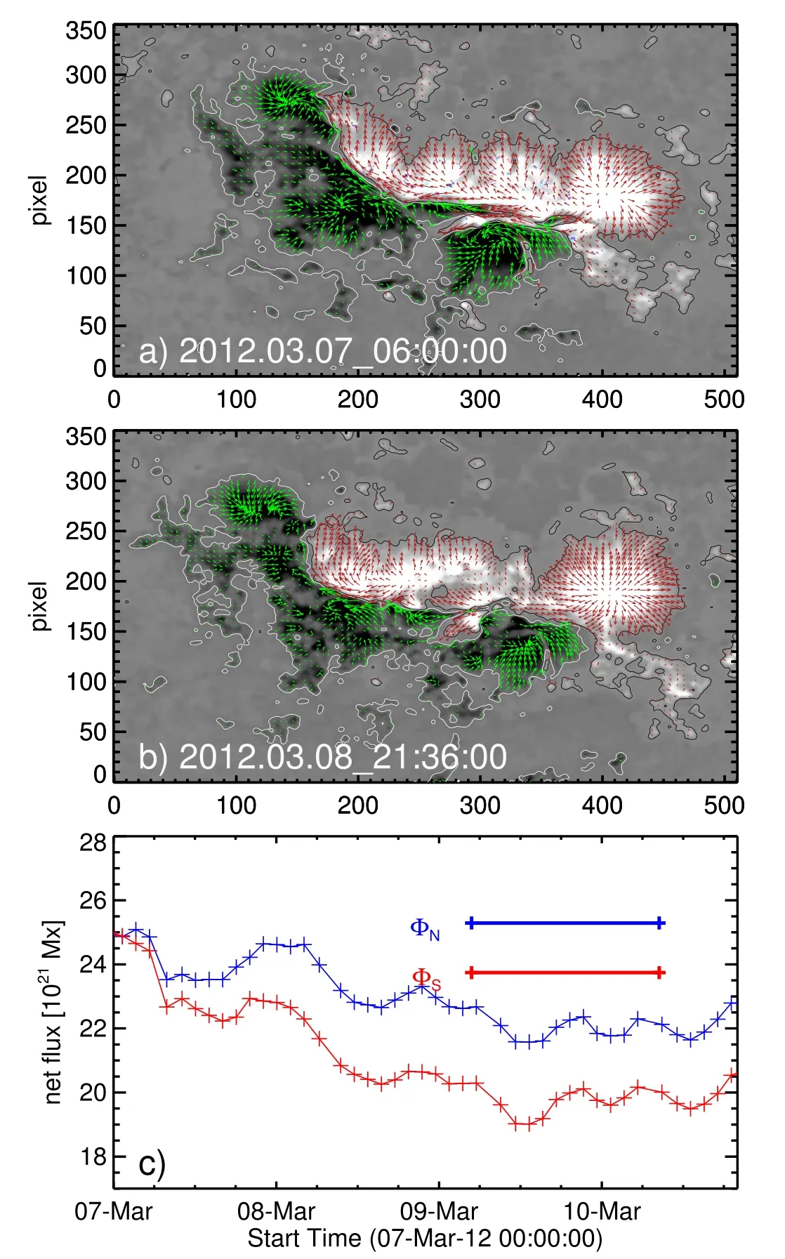
Figure 1.((a)–(b))HMI vector magnetic field observations of the AR 11429 at two different times in the evolution.The background image is the normal component Bz of the magnetic field with overplotted contours at ±120 G.Arrows refer to horizontal fields, (Bx, By), with their length being proportional to the magnitude Bh = Bx 2 + By2.The axis units are in pixels of 0 5.(c)Time evolution of the net flux in each polarity of the AR.
AR 11429 pre-emerged and appeared in the north latitudinal belt N17° as seen from the Earth view.Snapshots of vector field observations of AR 11429 at two different epochs of the evolution are displayed in Figure 1.These magnetograms reveal the presence of a large interface of opposite polarities referred to as the polarity inversion line(PIL).Over time,these polarities evolve with persistent shearing and converging motions.These motions might have led to continuous flux cancellations inferred from the time profile of the magnetic flux in the AR(Dhakal et al.2020).The coronal EUV images of the AR present a plasma loop structure resembling inverse-S sigmoidal morphology, which was modeled to show the presence of a twisted flux rope in the core of the AR(Vemareddy 2021).During the disk passage,the AR produced three major eruptive flares with CMEs of speeds exceeding 1000 km s-1.In this study,we consider 72 hr of AR evolution starting from 03:00 UT on 2012 March 7 by driving the initial condition with the time series of observational data via the MF method.After two days of evolution,the AR again produced an eruptive flare of M-class at 03:53 UT on 2012 March 9.This means that the magnetic evolution leads to storage of magnetic energy by building a twisted flux rope,and we aim to capture a similar evolution through MF simulations.
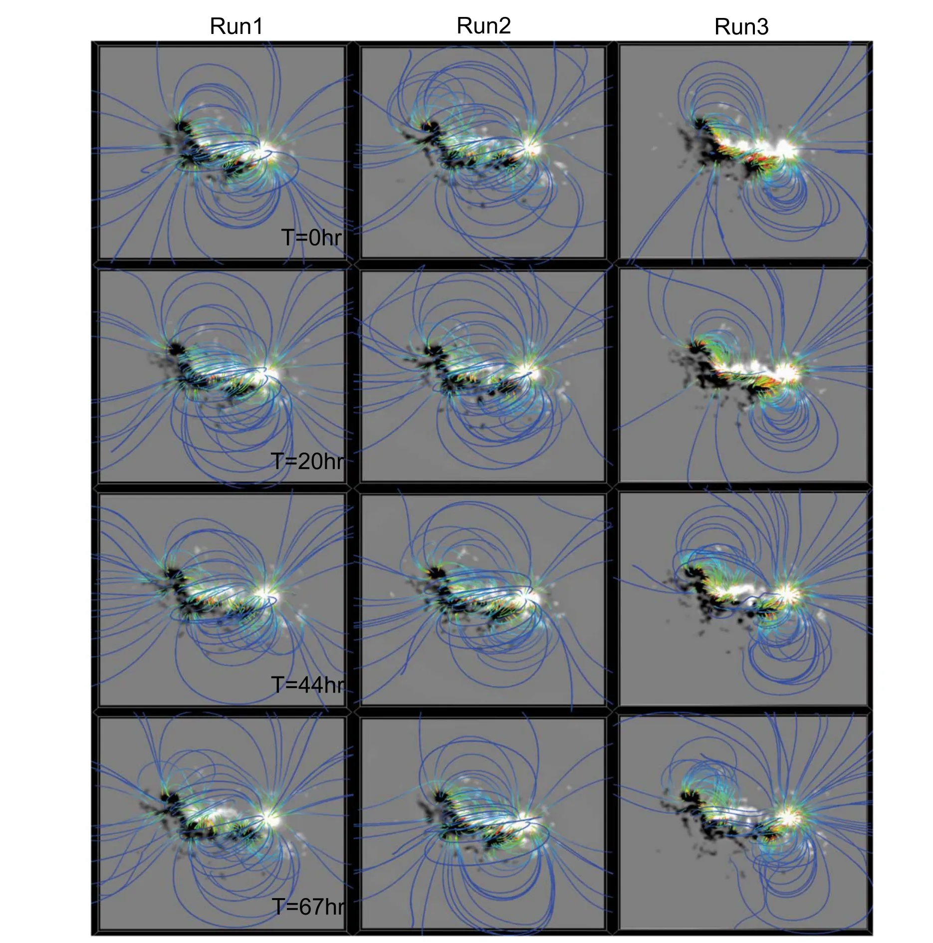
Figure 2.Magnetic structure at different epochs of the simulation:Run1(first column),Run2(second column)and Run3(third column).The background image is the normal magnetic field Bz at the photosphere(z=0)in gray shades together with magnetic field lines color-coded by their field strengths.In Run1 and Run2,the magnetic field evolves to be mildly sheared as it is not much different from the initial condition.However, the magnetic structure in Run3 is highly sheared and resembles an inverse-S shape as a whole.(An animation of this figure is available.)
We perform three different MF runs with appropriate combinations of initial and bcs.Run1 is a simulation with the PF as initial condition driven by bc1 as described in Section 2.4.Run2 is the PF initial condition driven by bc2.A uniform average twist is derived from the vector field observations and is injected into the corona.In Run3,we drive the NLFFF as the initial condition with bc3.In this case, an ad-hoc assumption involved is that the magnetic fields decrease exponentially up in the corona, so the horizontal fields are reduced by a factor c=0.7 and then used to prescribe the bottom boundary which is changing in time.The 3D magnetic fields of these runs are analyzed and the results are described in the following.
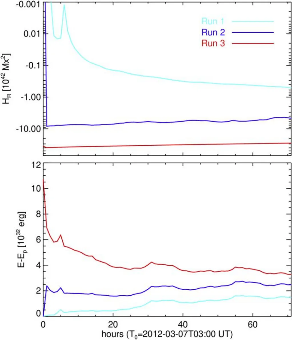
Figure 3.Time evolution of top: total magnetic helicity H, bottom: total magnetic energy E for Run1 (cyan), Run2 (blue) and Run3 (red).The start time of the simulation is 03:00 UT on 2012 March 7.
The simulated 3D magnetic field of the runs is visualized with the VAPOR software (Li et al.2019).In Figure 2, the magnetic structure of the AR is displayed by tracing the field lines at different epochs of the evolution.The foot point locations of the depicted field lines are chosen with a bias based on a variable such as horizontal magnetic field (Bh) and total current magnitude Jtot.The initial field structure is shown in the first row panels.Even the shearing motions of opposite polarities, the magnetic structure in Run1 exhibits less nonpotential behavior without much difference from the initial field.We expect that this is due to no magnetic twist information being pumped from the boundary which, even with horizontal motions, deforms the initial PF state insignificantly.The magnetic structure in Run2 evolves to a little more sheared state since we assume the boundary field to be linear force free.Being already in a non-potential state, the magnetic structure in Run3 appears highly sheared and resembles an inverse-S shape as a whole.It can be noticed that the shearedness increases with time because the twist information from the horizontal field is added to the driver field from boundary observations.An animation of the three runs together is available online for a better comparison of simulations.
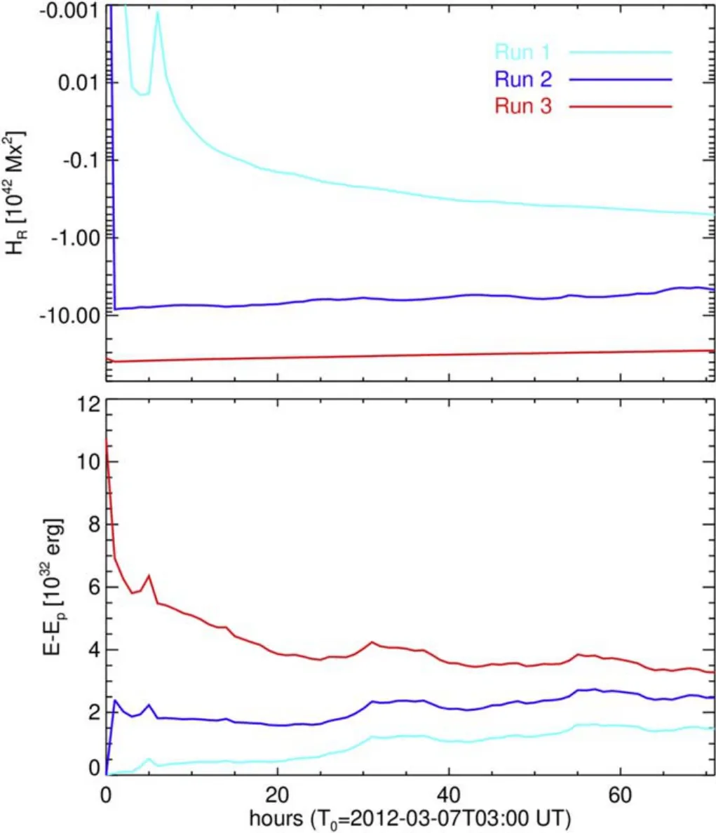
Figure 4.Time evolution of top: relative magnetic helicity HR, bottom: free magnetic energy Ef for Run1 (cyan), Run2 (blue) and Run3 (red).The start time of the simulation is 03:00 UT on 2012 March 7.
In addition,we have computed magnetic energy and helicity from the volumetric distribution of magnetic field above the AR and plotted the results in Figures 3 and 4 with time.Especially, to compare the coronal helicity budget, we derive the relative magnetic helicity (Berger & Field 1984) from the 3D simulated field as given by
Here the reference field is PF Bpand Apis the corresponding vector potential,which have the same normal component of the boundary field as that of the actual magnetic field under evaluation.The magnetic helicity H in Run1 increases in magnitude but is smaller by two orders(1040Mx2)compared to that obtained in Run2 and Run3, where the H value decreases over the course of the AR evolution by about 25%from the initial value.The H value varies from 39×1042Mx2in Run3 which is a typical value in terms of order of magnitude to produce a large-scale CME eruption.The relative helicity HRdiffers insignificantly from H since Hpis negligibly small and therefore it is not required to calculate HRseparately when using PENCIL CODE for such simulations.
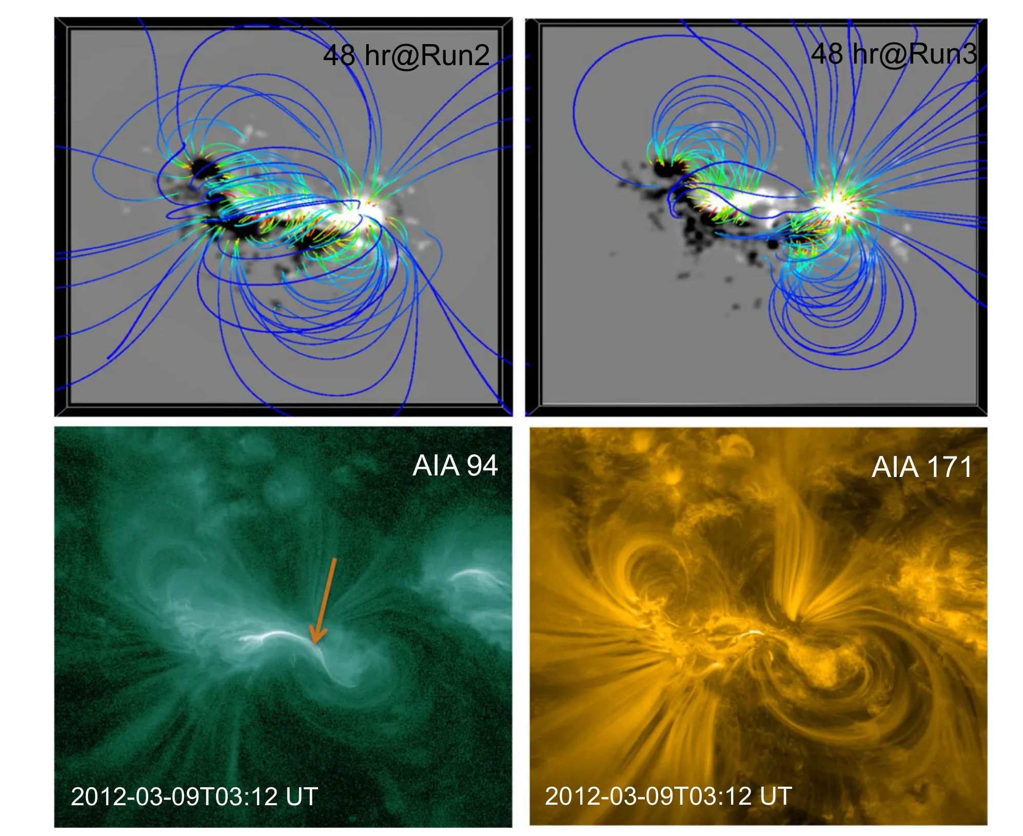
Figure 5.Comparison of magnetic structure with the coronal plasma tracers in AIA images of the AR 11429.Top row:Rendering of magnetic structure at 46th hr of Run2 and Run3.Bottom row:Images in 94 Å show predominant emission along the sheared PIL,which is a signature of a twisted flux rope,whereas 171 Å images present plasma loops as the lobes of the sigmoid.The magnetic structure in Run3 better resembles the sigmoid as seen in AIA 171 Å, however the core field is not twisted as much in flux to mimic the hot emission as seen in AIA 94 Å.
We note that the total magnetic flux as well as the average twist(αav)in the AR decreases with time(Dhakal et al.2020).The H increases due to shear motions alone which is below 1042Mx2in Run1, however, there is no additional increasing twist information in the horizontal field observations, and as a result the coronal helicity budget decreases in Run2 and Run3 from their initial values.Under these conditions,it is difficult to model the formation of twisted flux and its eruption.These types of ARs have to be treated with a provision to pump as much helicity as possible through boundary observations into the corona (Cheung & DeRosa 2012).
We have also evaluated the total and free magnetic energies.Given the 3D magnetic field in the computational volume, the free magnetic energy is calculated by
where Bpis the potential magnetic field.The total energy E decreases from 31×1032erg at the start of Run3 to 22×1032erg, which is following the total magnetic flux evolution as in Figure 1(c).This corresponds to a decrease of Ef/E from 20%to 15%.For Run2 and Run1,the E follows a similar trend with lower values compared to Run3.However, Ef/E increases to 10% for Run1 and to 15% for Run2 during the modeled evolution.In all these runs, the free energy is typically comparable to M-class flares, and shows a characteristic difference among the three runs performed with different boundary and initial conditions.
Finally, we also compare the magnetic structure qualitatively with the coronal imaging observations in EUV wavelengths.In the top row of Figure 5, we have displayed the rendering of magnetic structure at the time instance of 46th hr from Run2 and Run3.The snapshots at this time correspond to the CME eruption at 3:53 UT on March 9,for which the pre-eruptive AIA 94 and 171 Å images at 03:12 UT are displayed in the bottom panels of Figure 5.The plasma tracers in AIA 171 Å present two lobes;one of their legs is adjacent to the other on opposite sides of the PIL.This implies a highly sheared magnetic field resembling an inverse-S sigmoidal configuration (Green et al.2002;Vemareddy&Demóulin 2018).This kind of morphology is almost similar to the magnetic structure generated in Run3 compared to Run2.However,the predominant emission seen in AIA 94 Å along the sheared PIL refers to a twisted flux rope at the core of the sigmoid, which is not reproduced in the simulation.Previous MF simulations by Yardley et al.(2018)also showed a similar difficulty of generating twisted flux at the core;however,the lobes of the sigmoid and their evolution were reported to be well captured.Altogether, the MF simulation presented here is able to reproduce the dynamical evolution of the AR consisting of a highly sheared magnetic field globally that is able to launch CMEs.
4.Summary and Conclusions
We have performed the data-driven MF simulations of AR 11429.The numerical procedure of the MF simulation is implemented, for the first time, in PENCIL CODE, which is publicly available to serve a variety of astrophysical problems.In this case, we are required to use only a magnetic module,and the bcs have to be prepared from the observations of the AR under study in the form of vector potential, which then have to be fed to the bottom boundary layer as the simulation advances in time.The twisted magnetic field generated from the MF simulations may also serve as the initial conditions for the full MHD runs including plasma, where one intends to study the thermodynamic evolution of flaring plasma, as well as other aspects.Compared to Warnecke & Peter (2019b),where the helicity is injected directly at the boundary, this approach is much closer to the observed loop structure and hence is more self-consistent with photospheric input data.
We perform three different MF runs with appropriate combinations of the initial and bcs.In this work, we invented a way to invoke magnetic field observations to drive the coronal field.The key point is to work with vector potential A instead of magnetic field B without worrying about the divergence condition.However, there is a lot of difficulty in converting B to A and this is the first such effort.The simplest case is to drive the PF with the observed normal component of magnetic field, which cannot lead to a build up of a sheared coronal magnetic structure.The latter two combinations of the initial and bcs are meant to inject magnetic twist information obtained from the vector field observations of the magnetic field.We found that the already sheared field,further driven by the sheared magnetic field, will maintain and further build the highly sheared coronal magnetic configuration, as seen in AR 11429.The sigmoidal morphology exhibited by AIA images at the pre-eruptive time is better reproduced by the bc with twist information added to the vector potential which then drives the NLFFF since the AR is pre-existing with a non-potential magnetic field, even after the first eruption on March 7.The quantitative estimates of magnetic helicity and energy clearly show a marked distinction in these three runs, with the higher of these values corresponding to the complex and twisted nature of the magnetic field.
Although the global sheared configuration is reproduced,the core field does not take the form of twisted flux mimicking the hot plasma emission.The twisted flux along the PIL is not generated at small scales,which is a drawback to deal with MF simulations in this study, as was also the case in the previous such simulations (Yardley et al.2018).As a note, the AR 11429 is a decaying AR, so the input of magnetic twist from the observations is less significant to reflect in the driver field,which could be a reason for the decreasing free energy and magnetic helicity.Under these conditions, capturing the formation of twisted flux during the AR evolution is a challenge.In such instances, new approaches with certain ad hoc assumptions are required.Cheung & DeRosa (2012)derived the electric fields based on the time sequence vector magnetic field with free parameters that add the twist information proportionately to the observations.Instead of magnetic fields, the electric fields thus derived were used to drive the MF simulations and then study the formation of the twisted flux rope at the core and its further eruptions.Such simulations have recently been employed (Cheung et al.2015;Pomoell et al.2019) to study the formation of the twisted flux rope in the course of AR evolution and then its rise motion in a few ARs.Therefore, it is worth driving the MF simulations with electric fields, and our future reports will follow such investigations.
Acknowledgments
P.V.acknowledges the support from DST through Startup Research Grant.SDO is a mission of NASA’s Living With a Star Program.Field line rendering is due to VAPOR visualization software(www.vapor.ucar.edu/).The author also thanks Gherardo Valori for his insights on the construction of vector potentials.This project has received funding from the European Research Council (ERC) under the European Union’s Horizon 2020 research and innovation program(Project UniSDyn, grant agreement No.818665) (JW).This work was done in collaboration with the COFFIES DRIVE Science Center.We thank an anonymous referee for helpful comments and suggestions.
ORCID iDs
P.Vemareddy https://orcid.org/0000-0003-4433-8823
 Research in Astronomy and Astrophysics2024年2期
- Research in Astronomy and Astrophysics的其它文章
- A Fermi-LAT Study of Globular Cluster Dynamical Evolution in the Milky Way: Millisecond Pulsars as the Probe
- Application of Regularization Methods in the Sky Map Reconstruction of the Tianlai Cylinder Pathfinder Array
- Effect of Cosmic Plasma on the Observation of Supernovae Ia
- Variable Stars in the 50BiN Open Cluster Survey.III.NGC 884
- Free Energy of Anisotropic Strangeon Stars
- The Clumpy Structure of Five Star-bursting Dwarf Galaxies in the MaNGA Survey