Analysis of pseudo-random number generators in QMC-SSE method

Dong-Xu Liu(刘东旭), Wei Xu(徐维), and Xue-Feng Zhang(张学锋)

Department of Physics,Chongqing University,Chongqing 401331,China

Keywords: stochastic series expansion,quantum Monte Carlo,pseudo-random number generator

1.Introduction

The Monte Carlo method is one of the most popular algorithms in various science and technology fields,[1]and its key use is to produce many independent samples following a specific distribution.To simulate the quantum many-body system,various quantum Monte Carlo (QMC) algorithms have been invented and improved.[2]One of the most popular methods is the stochastic series expansion (SSE) method.[3-6]The target distribution is the partition function represented with a series expanded form

whereHis the Hamiltonian simulated andβ=1/Tis the inverse of the temperature.Then,the updating processes of the SSE algorithm specifically depend on the form of the Hamiltonian.However, all the random sampling processes require the pseudo-random number generator (PRNG).Therefore, it is clear that the performance of the QMC highly relies on the suitability of the PRNG.[7-9]

The PRNG can generate a lot of numbers that behave as though randomly distributed,[10]but the “pseudo” part of its name means the numbers do not originate from truly random physical processes, such as the quantum effect, thermal fluctuation, or chaos.However, because the sequence of the random numbers{s0,s1,s2,...,si,...}presents very low autocorrelation, it can still be used to simulate random processes.Usually,PRNGs working on a computer can be separated into the following steps: (i) defining the iteration function, which can calculatesi+1based on the constant parameters and previous numbersi; (ii) initializing the parameters of the iteration function and also the first numbers0(sometimes equal to “seed”, which is the specific initial condition of the iteration function); and (iii) calculating the random number with the help of the iteration function step by step.The PRNG is pseudo-random,so it has some intrinsic problems,such as the periodicitysp+n=snwith periodp, or the “lattice” structure that sometimes exists.[11]

The effect of PRNGs on the Monte Carlo algorithm has been studied in depth.For the classical Monte Carlo, different PRNGs were tested for various updating algorithms like Metropolis,Wolff,and Swendsen-Wang to guarantee accurate results and optimal performance.[12]Especially when simulating critical systems, inferior PRNGs can lead to incorrect outcomes.[13]When it comes to first-principle calculations and molecular dynamics simulations, which make use of the diffusion and variational quantum Monte Carlo methods, most PRNGs can provide correct results under one sigma error bar,except for some underperforming PRNGs like RANDLUX and the short-period linear congruential generator (LCG).[9,14,15]Meanwhile, the autocorrelation length and CPU time can be influenced by the choice of PRNG.[8]However, such analysis of PRNGs on the world-line QMC has never been considered,so becomes necessary.

In this paper, we test the performance of different types of PRNG on the simulation of SSE methods.A quantity called QMC efficiency is introduced to evaluate the performance quantitatively.After checking different variables in one- and two-dimensional Heisenberg models, we provide a table explicitly demonstrating that the LCG is the best.The paper is organized as follows: in Section 2,we briefly review the QMC-SSE algorithm and define the efficiency of QMC;in Section 3, we discuss the chosen PRNGs and the environment parameters of the computing platforms;in Section 4,the benchmarks of PRNGs are presented; in Section 5, we draw conclusions.

2.QMC-SSE method

whereaiandbilabel the type and position of the operators,andSnrepresents the operator sequences.The program of SSE includes three steps: initialization,thermalization,and measurement.

In the initialization step,the parameters of the PRNG are set, especially the seed, so that the results are reproducible.Meanwhile,the information of the lattice is constructed,such as the position of the bonds, the coordinates of the sites, the relative positions of different sites,and so on.The configuration of the operator sequence and the status of each spin are also initialized.Most importantly, the weights of the operators are calculated,as well as the corresponding possibility of transferring one operator to the others.This is directly related to the updating of the operator sequence.In the computer program,the initialization step is only executed once,so the consideration of its efficiency becomes unnecessary.

The configuration of the operator sequence living ind+1 dimensions is updated in both thermalization and measurement steps.The updating algorithms are different,[16-18]and they aim to produce independent samples more efficiently.In the thermalization step,the system is approaching the ground state during the updating.It can be taken as thermal annealing because the number of operators increases during the updating, which is equivalent to decreasing the temperature.The thermalization step should follow a single Markov chain,so it cannot be parallelized.

The ideal updating process makes the nearest Monte Carlo steps uncorrelated.However,in the real simulation,this is extremely hard to achieve for all the observables.To quantify the correlation between Monte Carlo steps,the autocorrelation function is introduced as follows:[19]

wheretlabels the Monte Carlo steps and is sometimes called Monte Carlo time.Then,the normalized autocorrelation function can be defined asΓ(t)=C(t)/C(0).Typically, the autocorrelation function is an exponential decay exp(-t/τ) at large time,so we can takeτas the autocorrelation time.This indicates the correlation between Monte Carlo steps will decay down to 1/e afterτsteps updates,so thatOiandOi+τcan be approximately taken as Markov process or uncorrelated.However, there is often more than one decay mode.Therefore, here we use the integrated autocorrelation time defined asτint=(1/2)+∑nt=1Γ(t).[19]

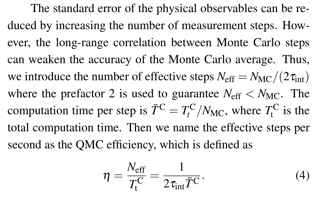
The inverse ofηis equal to the computation time per effective step,and we clearly find that a shorter autocorrelation time or computation time per step can give the QMC algorithm higher performance.This quantity is definitely different while considering different observables, because their autocorrelation times are determined by different modes of updating process.

3.PRNG and platform

The simplest but also fastest algorithm of PRNG is LCG,[21]which makes use of the linear congruence function as the iteration functionsi+1=f(si)=Mod(asi+b,p)with all coefficients being positive integer.It is obvious that the maximum period isp,and all the coefficientsa,b,andpshould be set within certain conditions so that the maximum periodpcan be reached.[22]Meanwhile,if the period is set to be the maximum of the 64-bit integer,the LCG algorithm can be strongly boosted by using the integer overflow.The integer overflow means the integer will throw the higher digits when the result is outside of the range after the operation,and it is equivalent to the function Mod().Although it is the fastest,the limitation of the digits of the register causes a serious problem that the period of LCG cannot exceed 264-1.

In 1998,Matsumoto and Nishimura broke this constraint and invented a random number generator called the Mersenne twister (MT), which is based on the matrix linear congruential method.[10,23]The most popular version is the MT-19937,which has a very long period of 219937-1.Then, Saito and Matsumoto introduced a new version of MT named the SIMDoriented fast Mersenne twister(SFMT),which is twice as fast as conventional MT, and its period is extended to be incredibly large 2216091-1.[24]On the other hand, another new version of the MT method named the well equidistributed longperiod linear generator (WELL) has better equal distribution and longer periods, and lower CPU time consumption.[25]The permuted congruential generator(PCG)was invented by O’Neill in 2014 and can provide a larger period with a smaller size register.[26]PCG can be taken as an improvement of the Xorshift method,which uses the shift and xor register method as the transform function.[26]Furthermore, we also consider another famous PRNG named KISS(after the“keep it simple,stupid”principle),which also has a long period 2123.[27]

The comparison of the PRNGs has to be implemented in the same computing environment.The CPU chosen is the Intel Xeon Gold 6420R processor(dual-channel,2.4 GHz,24 cores,and 35.75 MB high-speed L3 Intel Smart Cache),and the total memory is 256 GB(16×16 GB DDR4).The operating system is Linux CentOS 7.6.1810 and the program compiler is GCC 4.8.5.The optimization flags of the compiler are set as -O3 and -mAVX.The SSE algorithm is the direct loop method[6]and is written in C++ programming language without GPU boosting.The simulated system sizes of the one- and twodimensional Heisenberg models are set to be 500 and 24×24 under periodical boundary conditions, respectively.The inverse temperature isβ=1/T=10 (β=50 for calculating the winding numbers).As the free parameter of SSE,the energy shift of the diagonal vertex is set to 0.3.The number of measurement steps is as large as 105and the number of thermalization steps is half of that.

The Xeon processor utilizes the turbo boost technique,which will change the clock frequency of each processor.To rule out its influence, we use the clock() function in the〈time.h〉C library to count the system time and take an average of 1000 QMC runs (100 QMC runs for the two-dimensional case)with different initial seeds.

4.Results

First, the selection of the PRNGs definitely should not cause the QMC-SSE program to produce incorrect results.As mentioned before, some PRNGs (e.g., LCG) suffer from the“lattice” structure, and they may introduce serious problems,especially in the field of cryptography.Therefore, we examine various typical observables in one- and two-dimensional Heisenberg models and list them in Table 1.The largest deviation values are marked with colors.Their mean values are calculated by taking an average of many independent Markov chains with different initial seeds,and the standard errors with 2σ(95% confidence) are also shown.Here, the winding number is not considered in the one-dimensional Heisenberg model,because it is zero due to the absence of long-range offdiagonal order.From the numerical results,we can find there is no wrong result coming out with consideration of the statistical error.Thus, all the PRNGs listed are safe for QMCSSE,including the LCG,which is commonly used.However,it appears the SFMT algorithm with a larger period may easily cause an apparently larger deviation.

The efficiency of the algorithm can be reflected by the autocorrelation time.As mentioned before, the updating of different variables is determined by different modes of the transfer matrix.Therefore, we list the integrated autocorrelation times of all the observables in Table 2.We find the autocorrelation times of the observables are strongly different and sensitive to different PRNGs,but the deviations are small,which means the selection of PRNGs cannot strongly affect the autocorrelation between Monte Carlo steps.However,we notice that the PCG and KISS demonstrate much smaller autocorrelation times of winding numbers with larger standard errors.The reason has not been determined yet, but we think it may be related to the topological properties of the winding number.

The main goal of the PRNGs is to produce independent samples with low computing resource costs.It is common to take MT-19937 or LCG as the PRNG when writing the QMC code.In recent decades,PRNGs have been continuously under development and their performance has strongly improved;for instance, the SFMT is twice as fast as the MT series as mentioned on the homepage of SFMT.Contrary to the usual ways of thinking,the periods of PRNGs have less effect on the computation time,so a shorter period does not mean faster.In the QMC algorithm, the PRNGs only participate in the updating process and are not involved in the measurement.Thus, the computation time is estimated by running only diagonal and loop updates after the thermalization steps.In other words,the computation time affected by the PRNGs is not related to the observables.In Fig.1, we find that the influence of PRNGs is very serious in both dimensions.Counterintuitively, the SFMT with a smaller period costs a lot, especially in a twodimensional system.In contrast, SFMT-11213, 19973, and 86243 show very good performance.The LCG is widely used in SSE by Sandvik, and it is extremely good.KISS is also a notable alternative choice,and the computation cost of WELL series PRNGs is still fine.

Finally, we can calculate the QMC efficiency of all the observables listed in Table 3.Then,to simplify the qualification of the PRNGs,we define the benchmark score as follows:

whereηiis the QMC efficiency for thei-th observable withηMias the largest value among all the PRNGs, andnis the number of observables considered(e.g.,n=4 in 1D).Then,in one dimension,LCG,SFMT-11213,19937 and 86243 are the best choices.In comparison,LCG and KISS perform excellently in two dimensions.After taking an average of both dimensions,we recommend the LCG as the best PRNG in QMC-SSE.

Fig.1.The total computation time consumed for the(a)one-dimensional and(b)two-dimensional Heisenberg model within 105 Monte Carlo steps after thermalization.

Table 1.The numerical results of the one- and two-dimensional Heisenberg models calculated by the QMC-SSE method.The largest and smallest values are highlighted in red and green,respectively.

Table 2.The autocorrelation time of different variables of the one-and two-dimensional Heisenberg model calculated by the QMC-SSE method.The largest and smallest values are highlighted in red and green,respectively.

Table 3.The QMC efficiency and the scores of the QMC-SSE method.The recommended PRNGs are highlighted in red.

5.Conclusion

The performance of PRNGs in the QMC-SSE method is systematically analyzed in this work.The correctness of the algorithm is not ruined by the drawbacks of PRNGs,e.g.,short period,lattice structure,and so on.Meanwhile,the autocorrelation time is also less sensitive to the choice of PRNG,except for the winding number while using LCG and KISS.We find that the computation time contributes to the major impact on the performance.After introducing the QMC efficiency and benchmark score,we provide a strong recommendation for the LCG as the best PRNG in the QMC-SSE method.If the lattice structure is still a worry,KISS and SFMT-86243 would be alternative solutions.The selection of the best PRNG may be highly relevant to the type of QMC,but the process of analysis we have introduced here can also be borrowed as a standard procedure.

Program availability

The code used in this article has been published on GitHub at https://github.com/LiuDongXu-01/QMC RNG and is also openly available in Science Data Bank at https://doi.org/10.57760/sciencedb.j00113.00206.Download and decompress the code file QMC.tar.gz.Then, go into the decompressed folder.The readme file provides all the details on installing the program and how to use it.

Acknowledgments

Project supported by the National Natural Science Foundation of China (Grant Nos.12274046, 11874094, and 12147102), Chongqing Natural Science Foundation (Grant No.CSTB2022NSCQ-JQX0018),and Fundamental Research Funds for the Central Universities(Grant No.2021CDJZYJH-003).