工业过程关键指标预测的知识协同进化增强图卷积网络方法

牟天昊,邹媛媛,李少远

(上海交通大学自动化系,上海 200240;系统控制与信息处理教育部重点实验室,上海 200240)

1 Introduction

In industrial processes,precise control of key quality variables,such as product yield and element concentration,is essential.However,measuring these variables online is challenging due to harsh production conditions,costly analyzers,and lengthy laboratory tests[1].Consequently,key variable prediction methods have emerged to estimate these variables using easily measurable process variables [2-4].Key variable prediction methods outperform online analyzers and laboratory analysis in terms of fast response,low maintenance costs,high flexibility,and acceptable accuracy.As a result,they have gained substantial academic research attention.

Existing key variable prediction methods include knowledge-driven methods and data-driven methods[5].Knowledge-driven methods generally exhibit good interpretability and high accuracy.However,obtaining accurate process mechanisms for complex industrial processes is challenging in practical applications.On the other hand,data-driven key variable prediction methods require no prior knowledge[6].Among datadriven methods,the neural network(NN)models[7-9]show high accuracy and excellent nonlinearity approximation ability,rendering them the most popular key variable prediction methods in recent years[10-15].

Despite the above advantages,conventional NN models suffer overfitting and lack interpretability [16].To address these issues,researchers have explored the integration of prior process knowledge with NN models[17-20].Recently,the graph neural networks (GNNs)have gained significant attention as promising end-toend methods that effectively utilize graph knowledge,such as variable correlations and process flow topology.Among GNNs,the graph convolutional network (GCN) [21-22]has gained prominence,and several studies have applied the GCN in the process industry.For instance,in Chen et al [23],a structure-analysis-based GCN(GCN-SA)fault diagnosis method was proposed.It employed the SA for association graph construction and the GCN for integrating process data with prior knowledge.Similarly,in Wu and Zhao [24],process topology derived from the piping and instrument diagram(P&ID)was utilized as prior process knowledge,and a process topology convolutional network based on GCN was developed for fault diagnosis.In Chen and Ge [25],a soft sensor model based on graph convolution,stacked auto-encoder,and attention mechanism was proposed.

However,there are two inherent issues in the aforementioned GCN-based key variable prediction methods.Firstly,in current literature,process knowledge is treated as fixed prior knowledge which remains unchanged during GCN model training.Due to the high cost associated with constructing accurate knowledge for large-scale industrial processes,the prior knowledge is often coarse-grained and imprecise,thereby limiting the prediction performance of the final model.Second,existing methods cannot effectively extract and articulate the new knowledge embedded within the data,failing to gain further insights into the underlying process mechanisms.

Based on the aforementioned discussions,we propose an enhanced method called knowledge-based coevolution graph convolutional network (KBCE-GCN)for predicting key variables in industrial processes.Our approach addresses the two major issues by introducing an adaptive knowledge mechanism through graph exploration and knowledge filtering.During model training,the initially coarse-grained knowledge is continually updated,resulting in improved prediction accuracy and the discovery of new knowledge.Firstly,we construct an initial graph that represents the physical connections among process variables,units,and streams using the process flow diagrams (PFD).In this graph,the weights of edges are initialized through distance analysis.Secondly,we propose a training strategy with graph exploration,enabling simultaneous GCN model training and graph knowledge updating.This integration achieves high prediction accuracy while uncovering implicit knowledge within the data.Finally,we introduce a knowledge filtering mechanism based on the graph neural network explainer (GNNExplainer) [26],which eliminates insignificant new knowledge while complementing updated knowledge with prior knowledge.By knowledge filtering,knowledge complexity is reduced and knowledge consistency is improved.The contributions of this paper include:1)Proposing a novel data-knowledge-driven method for predicting key variables in industrial processes,encompassing graph construction,data preprocessing,model training with graph exploration,and knowledge filtering;2) Introducing adaptive knowledge to the conventional GCN prediction model.Through graph exploration and knowledge filtering,we discover new knowledge as well as achieve knowledge consistency;3)Validating the effectiveness of the proposed KBCE-GCN method using the benchmark debutanizer process.

The remainder of this paper is structured as follows.Section 2 presents the preliminaries including the definition of a graph and the fundamental concepts of GCN.In Section 3,we provide a detailed description of the KBCE-GCN method framework.The efficacy of our proposed method is demonstrated on the benchmark debutanizer in Section 4.Lastly,Section 5 concludes the paper.

2 Preliminaries

The definition of graph in this paper is in accordance with[27].

2.1 The definition of graph

2.1.1 The definition of graph

In computer science,a graph is a fundamental data structure utilized to represent pairwise relationships between objects.It is formally defined asG=(V,E),whereV={vi,i=1,2,···,n}represents the set of vertices or nodes andE={eij=(vi,vj)|vi,vj ∈V}represents the set of edges.Here,vi ∈Vdenotes a node in the graph andeij=(vi,vj)represents an edge originating fromviand terminating atvj.Nodeviand nodevjare considered adjacent if there exists an edgeeij ∈Econnecting them.The neighborhood of a nodevis defined asN(v)={u ∈V|(v,u)∈E}.

The adjacency matrixAis ann×nmatrix in which the elements indicate whether corresponding node pairs are adjacent or not.Specifically,Aij=1 ifeij ∈EandAij=0 ifeij/∈E.In addition,a graph may have node attributes specified as a node feature matrixX ∈Rn×d,wheredrepresents the dimension of node features.The node feature matrix can be regard as a dataset withnfeatures anddsamples,associated with the graphG.

2.1.2 The definition of weighted directed graph

A weighted directed graph is a graph in which edges have orientations and weights.An unweighted undirected graph can be regarded as a special case of weighted directed graphs where edge weights are restricted to the values of{0,1} and two inverse edges are present for every connected pair of nodes.It should be noted that the adjacency matrix of a weighted directed graph may not exhibit symmetry,and the element values within the matrix are not limited to{0,1}.

2.2 Graph convolutional network

Graph convolution is an operation performed on graphs that extends the concept of convolution from Euclidean space to non-Euclidean space of graph.It allows the extraction of representations from nodes and their neighboring nodes in a graph.An intuitive illustration of graph convolution is shown in Fig.1.

Fig.1 Convolution on Euclidean space (left) and convolution on graph domain(right)

Graph convolutions can be formulated as polynomials of the adjacency matrix or constructed via an extension of the Fourier transform to graphs.A detailed description of how graph convolution is developed can be found in the work of Hamilton[28].Kipf and Welling[22]proposed the GCN architecture,where a basic graph convolution(GC) layer is defined as follows:

whereHkis the matrix of node representations at layerkin the GCN,σdenotes an elementwise non-linearity such as rectified linear unit (ReLU) or sigmoid,Wis a learnable weight matrix,andis a normalized variant of the adjacency matrix with self-loops added,whereAis the adjacency matrix,Dis the corresponding degree matrix,andIis ann×nidentity matrix.

3 KBCE-GCN-based key quality variable prediction

3.1 Knowledge construction and data preprocessing

3.1.1 Graph construction

In an industrial process,physical connections among different process parts,such as production units and streams,provide insights into the arrangement of process components and the interdependencies of process variables.To extract this knowledge,Wu and Zhao[24]developed a graph construction method from process P&ID.This method requires no complex firstprincipal knowledge and significantly reduces the cost of graph construction.Innovated by [24],this paper constructs a graphG=(V,E),which describes the physical connections among process variables from the PFD.The nodes in the graph correspond to process variables,units,and streams,while the edges depict connectivity among these nodes.Moreover,the graph edges implicitly encode causal relationships among process variables.The flowchart illustrating the graph construction process is presented in Fig.2.Notably,the assignment of edge weights has not been addressed quantitatively and will be discussed in Section 3.1.3.

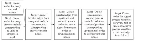
Fig.2 Main steps for graph construction

3.1.2 Data preprocessing

Generally,the historical data collected from the process consists of a data matrixand a label vectorY.

Then,the sliding window technique is employed to enhance data samples with time serial information.By sliding a window of sizetw,the sample of theith process variable at time steptis transformed into a time serial vector,as follows:

In graphG,each process variable node corresponds to a process variable in.Consequently,can be considered as the matrix of node features for the process variables nodes inG.However,the unit nodes and stream nodes are artificially defined and cannot be directly observed in the actual process.To satisfy the computational requirements of GCN,node features for unit nodes and stream nodes are artificially constructed by taking the average of node features of neighboring process variable nodes

wherevjis a unit node or a stream node,is the node feature for process variable nodeviat time stept,N(vj) is the neighborhood ofvj,Vpvis the set of process variable nodes,andis the node feature forvjat time stept.The input data matrix at time stept,denoted asXt,is computed by incorporating the node features for all process variable nodes as well as unit nodes and stream nodes,as follows:

From a graph perspective,the matrixXtcan be interpreted as an augmented matrix of node features at time stept.Specifically,each row inXtcorresponds to a node feature.These node features are designed to be one-hot-like vectors to capture the distinct physical meanings of the corresponding variables.From the viewpoint of the prediction model,Xtserves as the input matrix that is fed into the prediction model.

The label vectorY ∈RLcomprises values of the key quality variable collected fromLtime steps.Minmax normalization is applied to scale it to range[0 1].

3.1.3 Weights initialization

This study defines the distance between two nodes based on mean squared Euclidean distance

In equation(5),nodesviandvjcan be process variable nodes,unit nodes or stream nodes.x1,iandx1,jare the first node features forviandvj,respectively,as given by equation(2)and equation(3).The weight of the edge betweenviandvjis calculated by

whereσis the sigmoid function to scalew(vi,vj)into the range of[0 1].The initial adjacency matrixA0is given as

Following the steps in Section 3.1,a knowledgedata union{A0,Xt,yt}(t=1,2,···,L) which is necessary for the development of KBCE-GCN model is obtained,where{A0}is the knowledge component and and{Xt,yt}(t=1,2,···,L)is the data component.

It is worth noting that,in weight initialization,the selection of the distance measure is not strictly constrained,and empirical observations have shown that alternative distance measures,such as vector cosine distance,yield similar final prediction accuracy.Additionally,it should be emphasized that the initial graph knowledge is heuristically constructed as a starting point for the prediction model rather than aiming for optimal prediction performance.Some implicit variable relations,such as total heat supply constraint across process units,are not included in the initial graph.

Based on the above discussion,it becomes apparent that the development of an adaptive knowledge mechanism is necessary to enable knowledge mining and knowledge update during the training of the prediction model.Through the co-evolution of knowledge and the prediction model,one can expect improved prediction accuracy and enhanced knowledge consistency.

3.2 Model training with graph exploration

In this section,we introduce the procedures for training the GCN model with graph exploration.The core idea behind graph exploration is to consider the adjacency matrix as a trainable parameter and modify its element values while adhering to prior knowledge constraints.The network structure of the proposed KBCE-GCN model and framework of model training with graph exploration are shown in Fig.3.The model is composed of sequentially stacked multiple GC layers and multiple fully connected(FC)layers.

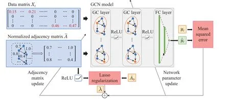
Fig.3 Framework of model training with graph exploration(the KBCE-GCN model comprises 2 GC layers and 2 FC layers)

In forward computing,the normalized adjacency matrixand the input data matrixXt(t=1,2,···,L) are fed into the model.At each GC layer,graph convolution is performed,by which the node representation of each node is calculated by aggregating node representations from neighbors as well as the node itself.The matrix of node representations at each GC layer can be obtained using equation (8) and equation(9)

In equation (8),the node representation matrix at the first GC layer isXt.In equation (9),Hkis the node representation matrix of GC layerk,ReLU denotes the ReLU activation function,is a weight matrix which mapsd-dimensional node representations tob-dimensional space,andKis the number of GC layers.The GC layers are stacked and the node representations are convolved layer by layer.The output of the last GC layer,i.e.,the node representation matrixHK,is a high-level representation ofXt.The matrixHKis then flattened and fed into the multiple stacked FC layers for regression.The output of each FC layer is given by equation(10)and equation(11)

In equation(10),flat is a function which flattens a matrix into a vector in row-first order.In equation (11),Op,are the output,weights and bias of thepth FC layer,andPis the number of FC layers.The output of the last FC layerOPis the predicted value of the key quality variable at time stept,denoted as.

After the feedforward computation,the loss function is computed.First,the prediction loss is measured by the mean squared error(MSE),given by

where Clip is a function that truncates matrix elements into the range of[0 1],and0is the normalized initial adjacency matrix.

In backpropagation phase,the Adam optimizer[29]is employed for parameter optimization.The network parametersis updated based onLaccalone.On the other hand,the knowledge parameterΘknow={} is updated based on a comprehensive loss function defined as

whereλis a hyperparameter which regulates the balance between prediction accuracy and knowledge complexity.

3.3 Knowledge filtering mechanism

Through graph exploration,new graph knowledge,including new edges and weights,is discovered.However,the quality of this new knowledge is not guaranteed and two key challenges arise in this process.Firstly,the adjacency matrix tends to become dense after black-box optimization,which contradicts the sparse nature of variable connections from a process mechanism perspective.Secondly,not all newly discovered edges and weights contribute equally to the model’s prediction,so it is important to differentiate their importance in terms of their impact on the final prediction.In this section,we propose a knowledge filtering mechanism to address these challenges.

Firstly,to identify the most crucial weights and edges for model prediction,we utilize the GNNExplainer model [26].In GNNExplainer model,a measure of importance is formulated by mutual information and an optimization problem is formulated by finding the most important subgraphGS.The optimization problem is given by

This optimization problem is reformulated as a masking problem of the original graph [26].The adjacency matrix ofGS,denoted asM,is computed by

To optimizeM,a loss function is defined as follows:

whereLdiffmeasures the prediction difference when the adjacency matrix changes from,Lsizeis a regularization term which limits the average size ofM,andLdispromotes discreteness inM[25].These three terms are defined as follows:

where 1n×nis a matrix of ones,and sgn denotes the sign function.The rationale behind the knowledge supplementation in equation(21)is that non-zero elements incorrespond to the structure of the initial graph,which is necessary to be included in the final adjacency matrix because the initial graph represents physical connections derived from the PFD and variable dependencies must depend on these physical connections.

To ensure process safeness,the adjacency matrixafter knowledge filtering requires additional validation by process experts before being utilized for online key quality prediction.

3.4 Pipeline of key quality variable prediction based on KBCE-GCN

The framework of key quality variable prediction based on the KBCE-GCN is illustrated in Fig.4.The main procedures are divided into an offline model training stage and an online model usage stage.

Fig.4 The framework of KBCE-GCN based key quality variable prediction

3.4.1 Offline model training stage

In the offline stage,historical data are collected as the process operates and stored in the process database.The PFD can be accessed from process experts.The historical data are preprocessed according to Section 3.1.2.An initial graph is constructed based on the PFD according to Section 3.1.1 and Section 3.1.3.Through data preprocessing and knowledge construction,the input data matricesXt(t=1,2,···,L),label vectorsyt(t=1,2,···,L),and the initial adjacency matrixA0are obtained.After that,the dataset{Xt,yt}(t=1,2,···,L) is split into a training set and a testing set.

The KBCE-GCN model is initialized as illustrated in Fig.3 and trained using the training dataset.During model training,graph exploration is performed.Following this,knowledge filtering is performed.If the decrease in prediction accuracy decrease is deemed unacceptable,a new round of training GCN model with graph exploration-knowledge filtering is initiated.Otherwise,model testing is conducted.

In model testing,the model is evaluated using the testing dataset.If the model performance is deemed satisfactory,the prediction model as well as the adjacency matrix,is saved and will be used for online usage.The adjacency matrix is separately exported for further process knowledge analysis.However,if the model performance is unsatisfactory,the model is redesigned and retrained.

It should be carefully pointed out that graph exploration and knowledge filtering have contrasting effects on prediction accuracy.Graph exploration mainly aims to increase prediction accuracy.On the other hand,knowledge filtering aims to maintain knowledge consistency and interpretability,which inevitably leads to a decrease in model prediction accuracy.Therefore,a thresholdβfor prediction accuracy decrease is used to indicate an acceptable decrease caused by knowledge filtering.If prediction accuracy decrease is deemed unacceptable,a new round of model training with graph exploration and knowledge filtering is started.Otherwise,the KBCE-GCN model is further tested.

3.4.2 Online model usage stage

In the online stage,the prediction model and the adjacency matrix are loaded.The process data are realtimely collected and preprocessed.Then real-time input data matrices are then fed into the KBCE-GCN model.The online predictions of the key quality variable are obtained by calculating the KBCE-GCN outputs.

4 Case study

4.1 Process description

The debutanizer column is a widely recognized benchmark platform for evaluating the performance of prediction models.In the refinery process,the debutanizer column is an important processing unit where propane (C3) and butane (C4) are separated from the naphtha stream.Its primary objective is to maximize the pentane(C5)content in the debutanizer overheads while minimizing the C4 content in the debutanizer bottom [2].The flowchart of the debutanizer column is depicted in Fig.5.Several hard sensors are installed in the column to capture real-time data of the process variables denoted as U1-U6.The description of these process variables is listed in Table 2.

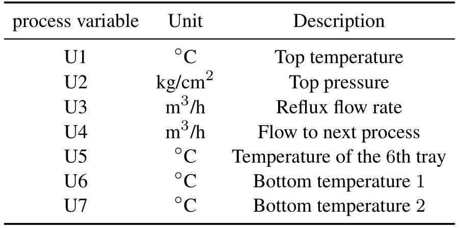
Table 2 Description of process variables in the debu-tanizer column

Fig.5 The process flow diagram of the debutanizer column[2]

Real-time measurement of the butane content in the bottom flow is crucial for enhancing control performance.However,the butane content is measured by a gas chromatograph on the overhead of the downstream deisopentanizer column,with a measuring cycle lasting 15 minutes and a time delay of 45 minutes.Consequently,it is necessary to develop an online prediction model.

4.2 Knowledge construction and data preprocessing

4.2.1 Intial graph for the debutanizer column

Following the steps given in Section 3.1.1,the initial graph for the debutanizer column is constructed as shown in Fig.6.

Fig.6 The initial graph constructed for the debutanizer column process

The initial graph consists of 5 unit nodes,4 stream nodes,and 8 process variable nodes,represented by blue,grey,and orange colors,respectively.It is noted that some streams,such as the bottom stream to downstream,are not included in the constructed graph because they are not directly related to any process variables.

4.2.2 Process data preprocessing

The process data of the debutanizer column can be temporarily downloaded from https://drive.google.com/drive/folders/1pwmfTs-U5JHzSs14XcT8DOiCR M7IBUjl,as mentioned in[30].The process data contains 2394 samples collected at a sampling interval of 15 minutes.It includes 7 variables,namely U1,U2,U3,U4,U5,U6,andy.U1 to U6 are process variables described in Table 2 andyis the bottom flow butane content,which is the key quality variable.

Previous research has demonstrated that the debutanizer column is a typical dynamic process [30-32].Therefore,key quality prediction models should not only predict on samples at the current time step,but also consider previous samples.Based on the practical experiments in [30],process variables are chosen as=[U1(t) U2(t) U3(t) U4(t) U5(t) U6(t) U7(t)y(t-4)],where U1(t)to U7(t)are process variables measured by real-time hard sensors,andy(t-4) is a historical key quality variable.

In data preprocessing,a window size of 8 time steps is chosen to account for the measuring delay.Consequently,samples of process variables are 1× 8 time serial vectors.On the other hand,samples of unit nodes(i.e.,reactor,overhead condenser,head flux pump,feed pump to downstream,reboiler) and stream nodes (i.e.upper flow of reactor,reboiler flow to reactor,reflux flow,and feed flow to downstream) are computed according to equation 3,which are also 1×8 vectors.After that,the input data matricesXt(t=1,2,···,2383)are computed according equation 4.Xthas the size of 17×136,with 17 rows and 17×8=136 columns.The label vectorYis of size 2383×1.The final dataset{X,Y}or{Xt,yt}(t=1,2,···,2383)is split into a training set and a testing set using a split ratio 4 : 1,resulting in 1907 samples for training and 476 samples for testing.

4.2.3 Graph weights initialization

Following equation(13)-(15)in Section 3.1.3,initial graph weights are obtained and the corresponding normalized initial adjacency matrix0is shown in Fig.7.

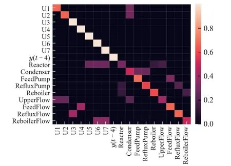
Fig.7 The normalized initial adjacency matrix

In Fig.7,sparsity is observed in the initial adjacency matrix.This sparsity arises from the graph construction process,which only considers physical connections derived from the PFD.As discussed before,the initial graph is necessary but insufficient for accurate prediction.Graph exploration is designed to solve this issue by supplementing the initial graph with new knowledge mined from process data.

4.3 Model structure,training parameters and evaluation criterion

In this paper,the proper number of GC layers is experimentally chosen as 2 to avoid the over-smoothing problem[33].The dimensions of node representations in the GC layers are set as 136 and 34,respectively.The output of the last GC layer with a size of 17×2 is flattened into a 34×1 vector,which is then fed into three stacked FC layers with a shape of[34,8,1].The output of the last FC layer corresponds to the predicted label.

Development for KBCE-GCN model follows the procedures outlined in Section 3.4.In the stage of training GCN model with graph exploration,the model is trained for 50 epochs using a minibatch size of 50 samples and a learning rate of 0.01.The coefficientλin the loss function is set as 0.1.Adam[29]optimizer is used for parameter optimization.In the knowledge filtering stage,the GNNExplainer is trained for 50 epochs using a minibatch size of 50 samples and a learning rate of 0.01.Adam[29]optimizer is used for mask matrix optimization,and the truncation thresholdαis set to 0.1.The thresholdβfor judging the acceptability of the performance decrease is set to 0.01 rooted mean squared error(RMSE).

In model testing,two commonly used evaluation criteria,RMSE andR2,are employed to evaluate the model performance.These criteria are defined as follows:

whereLtestis the number of samples in the test dataset,andis the average value of all labels in the test dataset.In general,a lower value of RMSE (close to 0) and a higher value ofR2(close to 1) indicate better model performance.

4.4 Experimental results

We compare the proposed method with four different prediction methods: deep neural network (DNN),GCN,supervised long-short term memory (SLSTM)[34],graph mining,convolution,and explanation framework with stacked target-related autoencoder (GMCE-STAE)[25].The DNN model comprises 1 input layer,3 hidden layers,and 1 output layer,with [2312,289,51,8,1]neurons,respectively.The GCN model consists of two GC layers and one hidden FC layer,with dimension of node representations chosen as[136,34].The hidden dimension of SLSTM is set to 90.In GMCE-STAE,the GC layer number is 1 and the STAE has 3 hidden layers.The hyperparameters of the models are listed in Table 3.The network structure and hyperparameters of DNN,GCN,and KBCE-GCN are determined through trial-and-error,while those for SLSTM and GMCE-STAE are determined by referring to[34]and[25].

Table 3 Hyperparameters of key quality prediction models

The simulation experiments were conducted on a PC with an Intel i5-6300HQ processor using Python3.7.Table 4 presents the test results of soft sensor models,obtained from 10 experiments with different random seeds.The prediction RMSE of the proposed KBCEGCN method is 64.3%～28.6%lower than other methods.Additionally,the KBCE-GCN method shows a 4.11%～0.10%higherR2index.These findings lead to the conclusion that the KBCE-GCN method exhibits superior prediction performance compared to other stateof-the-art methods.

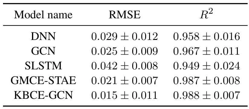
Table 4 Test results of key variable prediction models

Fig.8 illustrates the prediction performance of KBCE-GCN from four different perspectives.Fig.8(a)illustrates the prediction result sequence and shows that prediction labels track well with real labels.Fig.8(b)is the quantile-quantile plot of prediction results.It can be observed that the majority of data points cluster around the red 1:1 reference line.Fig.8(c)reveals that prediction errors are close to 0.Fig.8(d)showcases the histogram and probability distribution function(PDF)of the prediction errors.The PDF exhibits a narrow,spikeshaped distribution centered around zero and the histogram aligns well with a normal distribution.

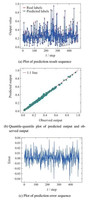
Fig.8 Prediction performance of KBCE-GCN

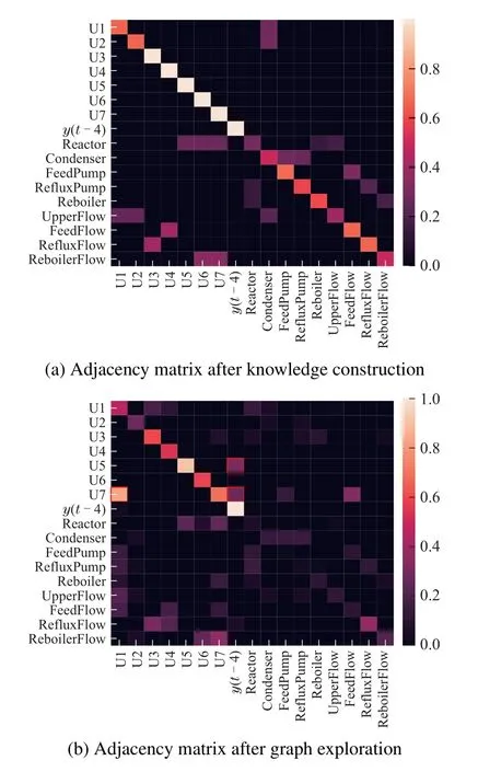
Fig.10 A comparison of adjacency matrices of three stages in KBCE-GCN development

There are three stages of graph knowledge during model development:knowledge construction,graph exploration,and knowledge filtering.To facilitate a comparative analysis,Fig.9 displays the heatmaps of the normalized adjacency matrices at each stage.Comparing Fig.9(a) and Fig.9(b),it is clear that graph exploration attenuates most edges among unit nodes and stream nodes,while preserving most edges among process variable nodes.Notably,graph exploration reveals three newly discovered connections,highlighted by red rectangles in Fig.9(b).The newly formed edge from U5(t) toy(t-4) is reasonable due to the fact that the 6th tray is the sensitive tray and the key quality variable (y) is controlled by regulating its temperature(U5).Similarly,the edge from U7(t)toy(t-4)is consistent with known physics as the bottom temperature(U7) directly influences the heavy component concentration in the bottom flow,thereby impacting the bottom flow butane concentration (y) through mass conservation.Moreover,since U5(t)and U7(t)are temperature variables within the same unit,they exhibit a high correlation.Overall,the three newly discovered connections through graph exploration demonstrate reasonable consistency with known process physics.

During the knowledge filtering stage,several edges deemed unimportant for key quality variable prediction or too weak were eliminated.Additionally,an edge from the reactor to the reboiler was added based on the initial adjacency matrix,as shown in Fig.9(b)and Fig.9(c).The decrease in prediction accuracy caused by knowledge filtering is 0.0023 RMSE,which falls below the acceptable threshold of 0.01.In conclusion,the proposed KBCE-GCN discovers new graph knowledge while maintaining a remarkable consistency with initial knowledge.

5 Conclusion

This paper proposes a KBCE-GCN method for industrial key quality variable prediction,which aims to overcome the limitations of existing GCN-based methods,including the high cost of constructing accurate prior knowledge and the lack of knowledge mining ability from abundant data.The method consists of knowledge initialization,graph exploration,and knowledge filtering.In the knowledge initialization phase,an initial graph is constructed based on the PFD.This serves as a reasonable starting point for the prediction model.In the graph exploration phase,new knowledge is discovered by maximizing prediction accuracy while adhering to prior knowledge.In the knowledge filtering phase,knowledge complexity is reduced and knowledge consistency is preserved by eliminating unimportant new knowledge and supplementing prior knowledge.Through the proper design of knowledge initialization,graph exploration,and knowledge filtering,a high-performance prediction model is obtained and new knowledge consistent with process physics is discovered.The proposed KBCE-GCN method is validated through experiments on a debutanizer column,demonstrating excellent prediction accuracy and the ability to obtain high-quality new knowledge.