The Existence of Domain Wall Solutions in Ambjørn-Nielsen-Olesen Theory

CAO Lei,CHEN Shou-xin1,

(1.Institute of Contemporary Mathematics,Henan University;2.School of Mathematics and Statistics,Henan University)

Abstract:The Ambjørn-Nielsen-Olesen(ANO)model arises from field theory,in the limiting BPS state,the ANO model is actually a domain wall model which is a basic construct describing a phase transition between two phases.In this paper,we derive a coupled second-order ordinary differential equations of the domain wall model.Then we establish the existence and uniqueness theorem for the domain solutions by using a dynamical shooting method for the parameter γ =1,and variational method for the parameter γ >0 and γ 6=1.

Key words:ANO model;domain wall;dynamical shooting method;calculus of variations

§1. Introduction

Ambjørn,Nielsen and Olesen first showed the relationship between non-Abelian vortex zero modes in the large magnetic flux limit and the magnetic instabilities.The earliest series results[25-26]about the existence of non-Abelian vortex are got from weak current vortex equation[1-4]and the series results were strengthened later[11,13].If the vortex is limited by the large magnetic flux[6-9],it becomes essentially a tube with constant magnetic field in the interior region separated from the vacuum by a thin domain wall.

Domain wall is a topological soliton in one dimension and describes a phase transition between two phases.In magnetism,magnetic domains are separated by a domain wall which also is a gradual reorientation of individual moments across a finite distance.Ne´el wall and Bloch wall are two typical types of domain walls.The sine-Gordon model governs the simplest domain walls which are derived from the Landau-Lifshitz magnetism theory.Besides,the sine-Gordon model often be regarded as the origin of both the Skyrme[20-23]and Faddeev model[16-18].

In this paper,we shall consider the Ambjørn-Nielsen-Olesen(ANO)model arising in the simplest non-Abelian U(2)–gauge field.In[5]the authors used a numerical method to get a domain wall solution.However,we will use mathematical method to strictly prove the existence and uniqueness of domain wall solutions.

The rest of our paper is organized as follows.In Section 2 we will introduce the ANO model and derive the mathematical structure which is a two-point boundary value problem of a coupled second-order ordinary differential equations.Meanwhile we state out main results.In Section 3,we derive a two-point boundary value problem of the ordinary differential equation from the coupled second-order ordinary differential equations for parameter γ=1,the existence and uniqueness of the solution is established by using a dynamical shooting method.In Section 4,considering the finite energy,we will introduce a variational method to establish the existence and uniqueness theorem of the coupled second-order ordinary differential equations for parameter γ >0 and γ 6=1.

§2.The Model and Main Results

We study from[5],for arbitrary coupling parameter e and g,the BPS Lagrangian action density of the ANO model arising in the simplest non-Abelian U(2)–gauge field is

where fµν= ∂µAν− ∂νAµ,fµν= ∂µAν− ∂νAµ,q is a charged scalar field,|q|2=Tr(qq†),†indicate conjugate transpose,Faµνis a non-Abelian gauge field and Dµis the non-Abelian covariant derivative.

As in the Abelian Higgs theory[10,19],in static two dimensions they possess the BPS reduction[5]

We construct a domain wall structure interpolating the Higgs phase and the magnetic phase by using the following ansatz

which renders the BPS equations(2.2)into

These are then reduced to the following coupled second-order equations in terms of q1and q2

where γ=g2/e2.

In[5],a numerical example is presented showing that the equations(2.8)-(2.9)possess a solution for γ=2 in a finite interval but there is no detailed explanation.In the following we will present a complete mathematical analysis and establish the existence and uniqueness theory of the equations(2.8)-(2.9)for γ>0.

Define new variables u1=ln|q1|2,u2=ln|q2|2and set ui→ ui+lnξ,i=1,2,then the equations(2.8)-(2.9)are reduced to

In the case of Higgs to Higgs phase,the boundary conditions of the equations(2.10)-(2.11)are

Then the equations(2.10)-(2.11)become

So the second equation in(2.13)gives us

where h lies between 0 and g.Thus we have g00=c(x)g where c(x)>0.Noticing(2.12)we get g(±∞)=0.So using the maximum principle we deduce g≡ 0.Thus we have

The same argument then shows f≡0.

Therefore(2.10)-(2.11)only have the trivial solutions,u1=u2=0.This means that there exists a trivial domain wall between two Higgs phases.Next we consider the other interesting case,Higgs to magnetic phase with the boundary conditions

When γ=1,the boundary value problem(2.10),(2.11)and(2.14)turns into a single one

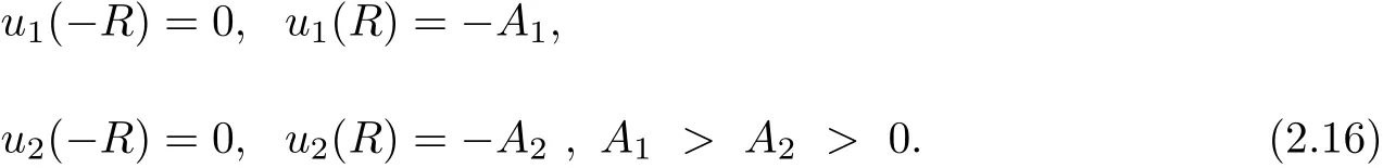
When γ >0 and γ 6=1,under the boundary conditions(2.14),the existence theorem of the solutions of the equations(2.10)-(2.11)becomes difficult.Due to space limitations,we do not elaborate too much here and will prove it in another article.We will consider the equations(2.10)-(2.11)in a finite interval(−R,R)with the boundary conditions

Our main results read as follows.

Theorem 2.1 There is only one solution fulfilling the two-point boundary value problem(2.15).

Theorem 2.2 The boundary value problem(2.10),(2.11)and(2.16)has a unique nontrivial solutions(u1,u2)on(−R,R).

§3. Proof of the Theorem 2.1

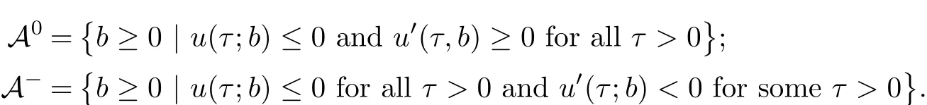
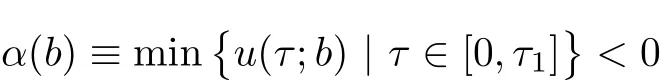
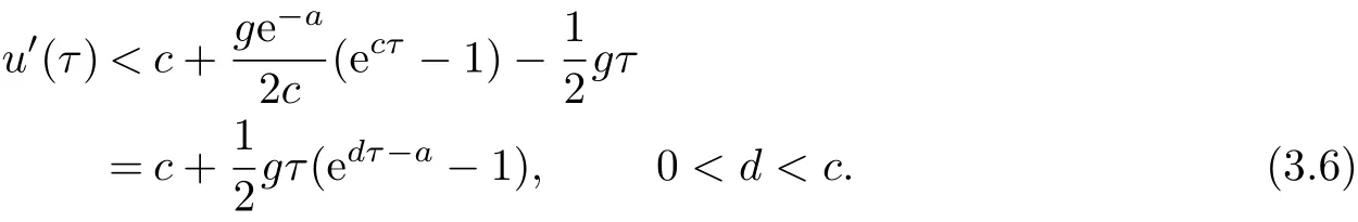
In this section we shall prove Theorem 2.1 using a dynamical shooting method suggested in[27].The shooting point is to be given somewhere in the middle of the interval−∞

In fact the choice of the initial point x=0 in(3.1)is arbitrary because the equation is autonomous.We first concentrate on the half x<0.

For convenient we now let x= −τ.Then in the region x<0 the system(3.1)becomes

In(3.2)we fix a>0 and vary b in the interval[0,∞).

Theorem 3.1 There exists a unique b>0 for any fixed a>0 so that the unique global solution of the initial value problem(3.1)satisfies u(−∞)=0,u(∞)= −∞.

To invoke a shooting argument,we use u(τ;b)to denote the solution of(3.2)(for fixed a>0)and set

Obviously,we have

Lemma 3.1 If b>0,the solution of(3.2)exists globally and satisfies u0(τ) ≤ 0 for all τ>0.In fact u decreases strictly for all τ>0.

Proof For τ>0 but τ is close to 0,we see that u00(τ)<0 from(3.2).So u0(τ)is decreasing and u0(τ)<0.If τ1is such a point makes u0(τ1)>0 and u(τ1)<0.Then there exists τ0∈ (0,τ1)so that τ0is a local minimum of u(τ)and u(τ0)<0.Such a situation contradicts the equation in(3.2).

To show that u is strictly decreasing,let τ1< τ2be such that u(τ1)=u(τ2).Then u(τ)=u(τ1)for all τ∈ (τ1,τ2).Applying the uniqueness theorem for the initial value problem of an ordinary differential equation we have u(τ)=0 for all τ≥ 0,which is false.The lemma thus follows.2

Lemma 3.2 For b sufficiently large,the solution of(3.2)will satisfy that u0(τ)≥ 0.In fact,u(τ)is strictly increasing for τ in the interval of existence and there is a point τ0so that u(τ0)>0.

Proof Let the interval of existence of the solution be[0,τ∞)with τ∞finite.If u(τ)<0 for all 0< τ< τ∞,then the solution can be extended to exist over an interval large than[0,τ∞),which is false.So either τ∞= ∞,u(τ)<0 everywhere or there is a point τ1>0 so that u(τ1)>0.We now show that when b is large enough the former case cannot happen.

In fact,integrate the equation in(3.2)we obtain

Hence for any fixed τ>0,we can choose b>0 sufficiently large to make u(τ)>0 which generate the case u(τ)<0 for all τ as claimed.

We continue to show that u(τ)is increasing.

Since b>0,u increases initially.Suppose that there is a point τ2so that u0(τ2)<0 in the interval of existence.Then,if u(τ2) ≥ 0,u will have a positive local maximum,violating the equation in(3.2).Thus u(τ2)<0 is the only possible situation.Of course,u(τ)<0 for all τ∈ [0,τ2],because otherwise we would have another nonnegative local maximum which is impossible.

Now we have τ1> τ2because of u(τ1)>0.The assumption u0(τ2)<0 implies that u has a negative local minimum in the interval(τ2,τ1).This violates again the equation in(3.2).

Therefore,we must have u0(τ) ≥ 0 for all τ∈ [0,τ∞).In view of the proof of Lemma 3.1 wee see that u strictly increases and Lemma 3.2 follows.

We know from Lemma 3.1 that 0∈A−and Lemma 3.2 that A+⊃(0,c)for c>0 sufficiently large.In the following discussion,we aim to prove that A06=∅.Such a result leads to solution of the original”two-point” boundary value problem(3.1).

Lemma 3.3 The set A+and A−are both open in[0,∞).

Proof Let b ∈ A+,τ1be such that u(τ1;b)>0.By the continuous dependence theorem we see that,u(τ1;c)>0 for c close to b.

In order to show that A−is also open,we need to distinguish two cases.

case(i):u0(0)=b>0.Hence,there is a point τ0>0 so that u0(τ0)=0.Clearly,u(τ0)<0,otherwise it contradicts the uniqueness theorem for ODEs.Then(3.2)gives u00(τ0)<0,which shows τ0must be a local maximum point.Since there can never be any local minimum point we see that

Let τ1> τ0.Then u0(τ1;b)<0,u(τ1;b)<0.For c close to b continuity says that

However,since it is easy to verify that u0(τ;c)<0 for all τ≥ τ1,we see that u(τ;c)<0 for all τ≥ τ1.On the other hand,since

continuously dependents on b,so when c is close to b,we also have α(c)<0.

In summary,when b>0 and c is close to b,we have u(τ;c)<0 for all τ≥ 0 and u(τ1;c)<0 for some τ1>0.Thus b is an interior point of A−.

case(ii):u0(0)=b=0.In this case we need to show e2ξ(e−a−1)<0 when c>0 is small.Then u00(τ)<0 for τ>0 small,this also shows that u0(τ)

Without loss of generality,we may assume τ0

We claim that when c>0 but c is close to 0,there is a point τ1∈ [0,τ0)so that u0(τ1)<0.Suppose otherwise that u0(τ) ≥ 0 for all τ∈ [0,τ0).Inserting this information into(3.5)and integrating,we obtain

We can see that for any fixed τ>0 sufficiently small,c will make the right hand side of(3.6)contradicting the assumption that u0(τ) ≥ 0 for any τ.So the claim u0(τ1)<0 for some τ1∈ [0,τ0)follows.

Consequently,there is a point τ2:0< τ2< τ1< τ0so that u(τ2)<0 and u0(τ2)=0.Using Lemma 3.1 we see that u0(τ)≤ 0 and u(τ)≤ u(τ2)<0 for all τ≥ τ2.This proves that u(τ)<0 everywhere.Combining this result with u0(τ1)<0 we arrive at the conclusion that c ∈ A−.

Lemma 3.4 The set A0is nonempty and closed.

Proof This is obviously a consequence of the connectedness of[0,∞).

Until now,we can assume b∈A0.Of course b>0 in view of Lemma 3.1.By definition of A0the corresponding solution u(τ)=u(τ;b)satisfies u ≤ 0 and u0≥ 0 everywhere.we easily see that u(τ)<0 for all τ using the uniqueness theorem for ODEs.Inserting this information into the equation in(3.2)we see that u00<0,u0>0,and u0decreases strictly for all τ>0.In particular,u(τ)(τ>0)is concave down and the limit

exists and is finite.Of course≤ 0.Besides,since u00<0 and 00,we obtain

exists and 0≤u1∞

The monotonicity of u(τ)implies u0∞=0.This immediately give us=0 because otherwise the lower bound u0(τ)>u1∞>0 would result in the false statement= ∞.

Lemma 3.5 There is only one point in the set A0.

Proof Let b,c ∈ A0,then v(τ)=u(τ;b)−u(τ;c)satisfies the boundary condition v(0)=0,v(∞)=0,and the equation Using the maximum principle,we have v=0.In particular,b=c.

Returning to the original variable x= −τ,we have derived a solution to problem(3.1)satisfying

Furthermore,in(3.1)with x>0,since a,b>0,we see that u00(x)<0 for x>0 small,which makes both u(x)and u0(x)decrease even further.Hence,for all x>0,u(x),u0(x),u00(x)<0.Such a fact leads to the direct consequence

Therefore Theorem 3.1 is obtained.We get a unique solution u to the initial value problem(3.1)exists over−∞

In other words,theorem 2.1 is established.

§4. Proof of the Theorem 2.2

In this section we aim to find solutions of the equations(2.10)-(2.11)under the boundary conditions(2.16).We will use a variational method as in[12]to prove Theorem 2.2.

Equations(2.10)-(2.11)can be written as

so that λ1=2γ, λ2=2 are two eigenvalues of Γ.It is easy to see(4.1)is the variational equations of the energy functional

where k·kp(p≥ 1)means the integral norm kfkp

To proceed further,we consider the problem on Sobolev space W1,2(−R,R)with the norm and using C(−R,R)to denote continuous function on(−R,R)whose norm is

then we have

For the positive definiteness of Γ−1,we yield the lower bound

where u stand for one of ui,i=1,2,with u=u+−u−,u+=max{u,0},u−=max{0,−u}.Then(4.7)can be written as

First,using the inequality

This shows that J(u+)is well behaved.On the other hand,from the fact that then we can estimate J(−u−)as follows:

To proceed,we recall Gagliardo-Nirenberg inequality in one dimention

where C1,C2>0 are constants.Using this result,we arrive at

which also shows that

where C3>0 is constant.That is to say

In fact,by virtue of(4.8)-(4.11),we see that

Consequently,inserting(4.6)and(4.12)into(4.3),we get the energy lower bound

which gives the coerciveness of the functional I(u1,u2)over W1,2(−R,R).

We introduce the admissible set as

Moreover,since W1,2(−R,R)⊂ C(−R,R),we have(,)→ (u1,u2).Besides,we can also assume I(,)≤σ+1,∀n,then we obtain

Now,we consider the optimization problem

where C>0 is constant independent of n.In view of(4.16),we know(x)→0 uniformly when x→−R and un1(x)→−A1uniformly when x→R.Similarly,(x)→0,(x)→−A2uniformly when x→ −R,x→ R respectively.By the weak semicontinuity of I(u1,u2)over W1,2(−R,R)×W1,2(−R,R),we obtainThat is,(u1,u2)solves(4.14).The strict convexity of I says that such a critical point of course a solution of I is unique.