
Detection of Oscillations in Process Control Loops From Visual Image Space Using Deep Convolutional Networks
2024-04-15 09:37TaoWangQimingChenXunLangLeiXiePengLiandHongyeSu
Tao Wang , Qiming Chen , Xun Lang , Lei Xie , Peng Li , and Hongye Su ,,
Abstract—Oscillation detection has been a hot research topic in industries due to the high incidence of oscillation loops and their negative impact on plant profitability.Although numerous automatic detection techniques have been proposed, most of them can only address part of the practical difficulties.An oscillation is heuristically defined as a visually apparent periodic variation.However, manual visual inspection is labor-intensive and prone to missed detection.Convolutional neural networks (CNNs),inspired by animal visual systems, have been raised with powerful feature extraction capabilities.In this work, an exploration of the typical CNN models for visual oscillation detection is performed.Specifically, we tested MobileNet-V1, ShuffleNet-V2,EfficientNet-B0, and GhostNet models, and found that such a visual framework is well-suited for oscillation detection.The feasibility and validity of this framework are verified utilizing extensive numerical and industrial cases.Compared with state-of-theart oscillation detectors, the suggested framework is more straightforward and more robust to noise and mean-nonstationarity.In addition, this framework generalizes well and is capable of handling features that are not present in the training data, such as multiple oscillations and outliers.
I.INTRODUCTION
OSCILLATION, which is the primary manifestation of deterioration of control performance, is still one of the most frequent problems in process industries [1]–[3].If not handled in time, it may lead to a decline in product quality,waste of raw materials and energy, and accelerated aging of equipment, which may directly impact the profitability and safety of the plant [4]–[6].The removal of oscillations means less variability in process variables, resulting in stable economic benefits for the production process [7].The prerequisite for removing oscillations is oscillation detection.However, a typical process industry is quite complex and may contain hundreds to thousands of control loops, so manual monitoring can be costly and prone to missed detection [8].In contrast, an automatic strategy is preferred.
Many automatic oscillation detectors have been reported over the past 30 years.The first algorithm for oscillation detection, which is based on integral absolute errors (IAEs)between successive zero-crossings, was proposed by Thornhillet al.[9], [10].In addition to this time domain approach,Yanet al.[11] proposed a detector by extracting repetitive patterns from the time series based on the hidden Markov model.Due to the periodic nature, oscillations may be more intuitive in the frequency spectrum.In light of this, frequency domain methods have been developed in succession.In an earlier study, Zhanget al.[12] developed a method based on the discrete Fourier transform and the Raleigh distribution to detect multiple oscillations in the presence of mean-nonstationarity.Recently, a novel framework for detecting oscillations using both time and frequency domain knowledge was proposed by Ullahet al.[13].
In general, the above methods are intuitive and easy to implement in engineering.However, most of them are susceptible to noise and disturbances.To tackle this challenge, methods based on the auto-covariance function (ACF) have been proposed.Miao and Seborg [14] first used ACF for oscillation detection, by defining the ACF decay ratio as the indicator.Recently, Thornhillet al.[15] devised a metric of ACF zero-crossing regularity, which is capable of detecting multiple oscillations by combining ACF with a band-pass filter.Following this work, Naghoosi and Huang [16] developed an improved technique to detect multiple oscillations directly without additional filtering.
Although ACF-based methods have good robustness to noise, their practicality to handle multiple oscillations and mean-nonstationarity is quite limited.The wavelet domain and decomposition-based methods can effectively handle the above complex plant data.On the basis of the wavelet transform (WT), a straightforward method for oscillation monitoring was presented by Naghoosi and Huang [17].Subsequently, Bounouaet al.[18] proposed an improved empirical WT method based on detrended fluctuation analysis to accurately extract the oscillating modes.We highlight that those methods based on the wavelet analysis are more accurate,however, at the expense of higher parametric degrees of freedom.
Most decomposition-based methods were developed inspired by related time-frequency analysis techniques in the field of signal processing, such as empirical mode decomposition [19], intrinsic time-scale decomposition [20], variational mode decomposition [21], and local mean decomposition(LMD) [22].The above methods are highly adaptive and can effectively cope with multiple oscillations and mean-nonstationarity in nonlinear processes.However, they assume that the investigated signal satisfies strict separation conditions in the time-frequency domain, and are therefore susceptible to mode mixing and low resolution in practical applications [4], [23].
In addition to the above reviewed methods, some emerging techniques, such as linear predictive coding [24], and machine learning [25]–[28], have recently been introduced.Notice that the ease of implementation of these methods remains to be further investigated.
In summary, all the methods reviewed above can only address part of the practical difficulties since most of them are rule-based [28].Therefore, there is a need to develop a method that is not bounded by specific rules for control loops of various data features.Here, we revisit the definition of oscillation.A widely accepted definition was presented by Horch [29], who designated oscillation as a periodic variation that is not completely hidden in noise, in other words, visible to the human eyes [7], [30].This definition suggests that loops containing oscillatory behavior are visually apparent.However, there is no work at the visual level yet that explores oscillation detection following the definition of oscillation.Although manual visual inspection provides highly intuitive detection results, it is not recommended for engineering applications due to its labor-intensive nature.
The presence of convolutional neural networks (CNNs), a representative of deep learning, provides a solution to detect oscillations from a visual perspective since they have proven successful in computer vision tasks [31]–[33].Given this, a framework based on the CNN models is explored, and featured by the following steps.First, the artificially generated process data are preprocessed through two stages, namely imaging and normalization.Following that, the preprocessed data are utilized to train four typical CNN models containing MobileNet-V1 [34], ShuffleNet-V2 [35], EfficientNet-B0 [36]and GhostNet [37].Finally, these trained models are used to carry out oscillation detection.The main contributions and advantages of this work are summarized as follows.
1) A framework for visual oscillation detection using typical CNNs is proposed and explored.
2) Due to the capabilities of powerful feature extraction of CNNs, the proposed framework can effectively handle multiple and time-varying oscillations in the presence of noise and mean-nonstationarity.
3) The CNNs used are all from typical networks in the field of deep learning, which are easy to implement.
4) The framework can be updated to process new oscillation problems with additional training data.
The rest of this paper are organized as below.Section II presents the details of the generation of artificial data and the structure of CNNs.Then, the process of using CNNs to achieve oscillation detection visually is elaborated in Section III.In Section IV, the effectiveness of the proposed framework is demonstrated by representative numerical experiments.Section V discusses the limitations of this framework and leads to future work by visualizing the detection results.Finally, conclusions are drawn in Section VI.
II.PRELIMINARIES
The effective execution of the proposed framework relies on two crucial prerequisites: the training data and the construction of the CNN models.In this section, their technical details will be introduced separately.
A. Generation of Artificial Data
The availability of big data and advancements in hardware are the main reasons for the success of CNNs [32].However,confidential and strategic issues make industrial data (especially those containing fault information) difficult to obtain in large quantities.Even when data is available, numerous issues are still to be solved, e.g., data cleaning, and the time-consuming task of data labeling.An alternative and successful solution–artificial data, was proposed by Dambroset al.[28].They pointed out that the generated data served for oscillation detection should obey the following rules: 1) The artificial data must be as similar as possible to the industrial (oscillation) data; 2) The artificial data must have examples from processes with different dynamics, configurations, and characteristics.
Accordingly, the generated data should have the following features: 1) Oscillatory and nonoscillatory examples of different lengths; 2) Noise and disturbances with different amplitudes; 3) Oscillatory time series with different numbers of oscillation periods; 4) Oscillatory time series with different waveforms, i.e., sine, triangle, and square waves, respectively;5) Waveforms smoothed with different intensities, approximating the oscillatory time series filtered by the process;6) Part of the oscillatory time series is time-varying with different intensities.
Dambroset al.[28] have defined a set of variables that obey various distributions for generating artificial data, which are listed in Table I.The value of each variable is a random number generated based on the probability density function of the corresponding distribution.More details on this can be found in [28].
As depicted in Table I, both noise and disturbance are originated from Gaussian white noise, whose magnitudes are determined byNvarandDamp, respectively.In addition, to mimic the industrial situation, both the disturbance and the oscillation need to be smoothed.More specifically, the disturbance is smoothed by the following transfer function:
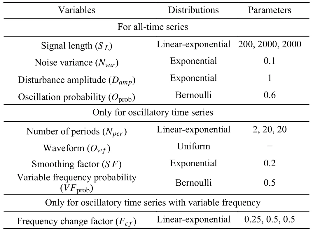
TABLE I THE VARIABLES USED TO GENERATE ARTIFICIAL DATA
while the oscillatory component is smoothed by the following transfer function:
The amplitudes of all oscillatory time series are set to be 1 to ensure the validity of variablesNvarandDamp.For frequency-invariant oscillation, its frequencyf0is determined by variablesSLandNper.On the contrary, the frequency seriesf(t) of the time-varying oscillation is calculated byf0andFc f.The detailed procedures of artificial data generation are given in Algorithm 1.
B. Convolutional Neural Networks
CNN is a type of network with a multilayer structure inspired by the animal visual system [38], [39].It can sufficiently exploit spatial or temporal correlation in data and is considered one of the best learning algorithms for understanding image content [32].Numerous variants of CNN architectures have been proposed in the past.However, their primary components are very similar [40].Typically, a CNN consists of four main components, namely, convolutional layers, pooling layers, fully connected layers, and activation functions,where Fig.1 visualizes its general architecture for image classification.
CNNs have remarkable attributes such as automatic feature extraction, hierarchical learning, and weight sharing, where the critical step is convolution [32].A convolutional layer is composed of a set of convolutional kernels that are used to generate various feature maps.However, the feature map after convolution consists of diverse features, which tends to cause the overfitting problem.In view of this, the pooling layer is proposed to reduce the dimensionality of the feature map to prevent data redundancy.Furthermore, the nonlinearity in CNNs is realized through the activation functions, which help the network represent complex features.Finally, its high-level reasoning generally relies on fully connected layers, which are usually used at the end of the network.
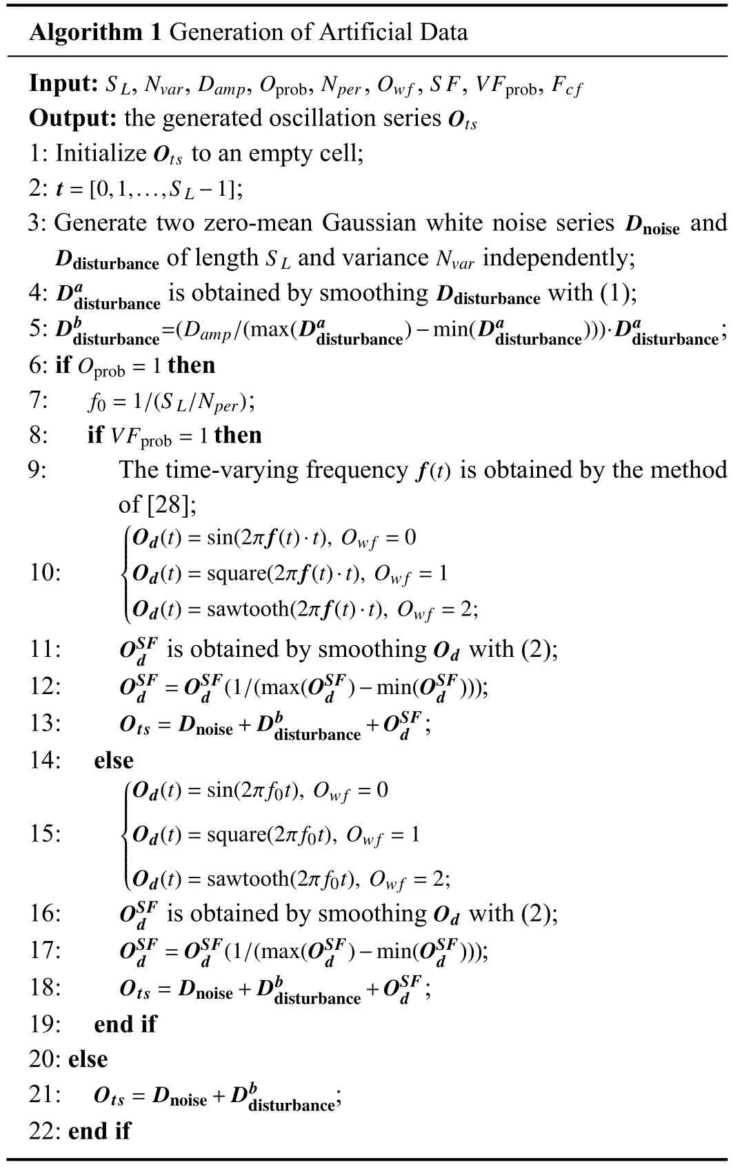
Algorithm 1 Generation of Artificial Data Input: , , , , , , , ,S L Nvar DampOprob NperOwfS FVFprob Fc f Output: the generated oscillation series Ots 1: Initialize to an empty cell;t=[0,1,...,S L-1]Ots 2: ;3: Generate two zero-mean Gaussian white noise series and of length and variance independently;Dnoise Ddisturbance S L Nvar Dad 4: is obtained by smoothing with (1);Db isturbance Ddisturbancedisturbance=(Damp/(max(Dadisturbance)-min(Dadisturbance)))·Dadisturbance 5: ;6: if then f0=1/(S L/Nper)Oprob=1 7: ;VFprob=1 8: if then 9: The time-varying frequency is obtained by the method of [28];■■■■■■■■■■■■■Od(t)=sin(2π f(t)·t), Owf =0 Od(t)=square(2π f(t)·t), Owf =1 Od(t)=sawtooth(2π f(t)·t), Owf =2;f(t)10:OSF d 11: is obtained by smoothing with (2);Od d =OSFd (1/(max(OSFd )-min(OSFd )))12: ;OSF disturbance+OSFd 13: ;Ots= Dnoise+Db 14: els 15:e■■■■■■■■■■■■■■■Od(t)=sin(2π f0t), Owf =0 Od(t)=square(2π f0t), Owf =1 Od(t)=sawtooth(2π f0t), Owf =2;OSF d 16: is obtained by smoothing with (2);Od d =OSFd (1/(max(OSFd )-min(OSFd )))17: ;OSF disturbance+OSFd 18: ;Ots= Dnoise+Db 19: end if 20: else Ots= Dnoise+Db 21: ;22: end if disturbance
III.METHODOLOGY
In this section, we focus on how to implement the detection of single-loop oscillation from a visual perspective.The general framework of the proposed solution is shown in Fig.2.As depicted, the proposed framework consists of three parts,i.e., data preprocessing, construction of the typical CNN models, and finally, detection of oscillations.
A. Data Preprocessing
The data preprocessing process is straightforward and consists of only two steps: process data imaging and pixel matrix normalization.For data imaging, the “plot” function in the MATLAB platform was used for simple imaging of sequences.The following points need to be satisfied when data imaging:
1) Distinguishable features can still be observed when the number of data points or periods of the oscillatory time series is extensive.
2) The original structure of the data cannot be destroyed.
3) The resolution size of imaging should match the performance of the experimental equipment, otherwise it may degrade the training speed of the model.
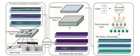
Fig.1.A general CNN architecture for image classification.
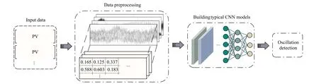
Fig.2.General framework of the visual methods.
Given the above, an appropriate image resolution of 200 ×2400 (height × width) is selected experimentally.
With respect to the normalization step, imaging pixels taking values between 0 and 255 are not suitable for CNN training, since CNNs are generally trained using smaller weight values for fitting.When the values of the training data are large integer values, it slows down the training process and additionally leads to the problem of overfitting.To tackle the issue above, we normalized the pixel matrix using the following operation:
where X(i)denotes theith input sample and X˜(i)represents the corresponding normalized result.
B. Models for Oscillation Detection
Although oscillation detection only needs a few classes of time series to be distinguished, it requires high image resolution.Therefore, if the chosen CNNs are of high complexity,then the high computational cost would be the main limitation.In contrast, lightweight CNNs show lower complexity and faster convergence, which are more suitable for application in oscillation detection.In view of this, here we explore the feasibility of four typical lightweight CNNs for oscillation detection, namely MobileNet-V1 [34], ShuffleNet-V2 [35], EfficientNet-B0 [36], and GhostNet [37].We highlight that these CNNs selected are the most popular neural networks available and their codes are open-source.Below is a brief description of these networks.
MobileNet-V1: MobileNet-V1 was proposed by Howardet al.[34] to balance the accuracy and complexity of the deep learning model.It is mainly constructed by the depthwise separable convolution block consisting of a depthwise convolution and a 1 × 1 convolution.Compared with the standard convolution, less computation and fewer number of parameters are required by the depthwise separable convolution.
ShuffleNet-V2: Maet al.[35] presented a more efficient network, ShuffleNet-V2, whose main body consists of two units that utilize “channel split” and “channel shuffle” operators to reduce network fragmentation.Additionally, element-wise operations are removed in each unit, thereby speeding up the computation of the model.
EfficientNet-B0: To balance the scale and performance of the network, Tan and Le [36] designed a baseline network(EfficientNet-B0) using a neural structure search and then scaled it with their proposed composite coefficient.Such composite coefficient is capable of scaling the depth and width of the network based on its predefined principles.Considering the requirement of fast and efficient detection, EfficientNet-B0 is chosen as one of our experimental models.
GhostNet: The feature extraction process of CNN generates a large number of feature maps, of which there are many similar ones.Therefore, Hanet al.[37] argued that redundancy in feature maps may be essential to a successful CNN.To this end, the Ghost module was designed to generate more feature maps through a simple linear operation.
The overall architectures of MobileNet-V1, ShuffleNet-V2,EfficientNet-B0, and GhostNet are attached to Supplementary material1Supplementary matenial of this paper can be found in links https://github.com/2681704096/Supplementary-materials-for-the-paper.git.for more detailed information.
C. Oscillation Detection
After building the CNN models, the next step is to train the models with artificial data for oscillation detection.There are two stages for training the CNNs: forward propagation and backward propagation.Specifically, the main goal of the forward propagation stage is to represent the input image with the parameters (weights and biases) of each layer.The forward output is then used to calculate the loss cost with ground truth labels.Based on the loss cost, the backward propagation stage calculates the gradient of each parameter using chain rules.Here, all parameters are updated according to the gradient and prepared for the subsequent forward calculation.
Mathematically, given a training set{(X(i),y(i))|i=1,2,...,N}, where X(i)denotes theith input sample,Ndenotes the number of samples in a batch, and y(i)is the label ofX(i)(using one-hot encoding), the output of the input sample through a series of linear and nonlinear operations (before the softmax operation) can be calculated as
where F(·) denotes the series of linear and nonlinear operations, andKdenotes the number of categories.The final step of forward propagation is the softmax classification operation,which converts the output of neurons into a probability distribution of classes.Concretely, the prediction resulttransformed by softmax is expressed as given by
The loss function plays the role of connecting forward propagation and backward propagation.Here, we selected the softmax categorical cross-entropy loss as the loss function, which is defined as
where θ denotes all relevant parameters used to construct the model (e.g., weight vectors and bias terms).
The update of parameters is related to the gradient direction,which aims to reduce the value of the loss function.For this purpose, gradient descent optimization algorithms are commonly used to quickly find the gradient descent direction.In this work, the stochastic gradient descent method with momentum is adopted as the optimizer because of its competitive generality [41].It can aggregate the velocity vectors in relevant directions so that the update of the current gradient depends on the historical batches.The process of gradient update is mathematically defined as
where γ and ηtdenote the momentum term (γisusually set to 0.9) and the learning rate, respectively.(X(t),y(t)) denotes a randomly picked sample.In practice, each parameter update is computed for a mini-batch rather than a single sample.
After sufficient iterations of both forward and backward propagation stages, the learning of the network can be stopped.Next, oscillation detection is achieved by feeding the preprocessed samples into the trained models.Concretely, a test sampleXtestis fed into the trained model, whose outputMo=[p1,p2,...,pj,...,pK]is obtained by combining (4) with(5), whereMois a vector containing the predicted probabilities of each class.Then, the class to which the sample belongs can be determined by obtaining the index valueIVof the maximum probability, as given by
IV.EXPERIMENTS AND RESULTS ANALYSIS
In this section, more information about the artificial and industrial datasets used for experiment is presented.Then,several metrics serving to evaluate the detection performance of all investigated CNNs are introduced.Finally, we give specific details on the implementation of the experiments.
A. Data Sets
1)Artificial Data: Artificial data was proposed by Dambroset al.[28] in 2019 (see Section II.A for details of data generation), and its corresponding download address can be found in[42].The dataset was generated by simulating the characteristics of industrial data and contains three classes, nonoscillation, regular oscillation, and irregular oscillation.In addition,the dataset contains 120 000 samples, with data lengths ranging from 200 to 24 064 points.However, this work only selected a random sample of 10 000 from the dataset because of its massive sample size and the limited performance of the experimental equipment.We also highlight that a small sample set better reflects the advantages of the proposed framework.Specifically, eighty percent of the selected samples were used as the training set, and the rest were used as the test set.Some simple examples of the dataset are shown in Fig.3.
2)Industrial Data: A benchmark dataset ISDB for oscillation detection and diagnosis was disclosed by Jelali and Huang [43].The data was collected from different industries such as commercial construction, chemical, pulp and paper mills, power plants, mining, and metal processing.Controller output and process output measurements for 93 control loops are contained in the dataset, and many of which are susceptible to noise, nonstationary trends, or other disturbances and anomalies.The oscillatory time series exhibit multiple, intermittent, and time-varying properties.Additionally, the dataset contains sequences that are clearly differentiated, ranging in length from 200 to 277 115 points and in amplitude from 0.0184 to 2303.4.Note that a portion of the data in this dataset are not explicitly labeled, however accurate data labels are required in subsequent experiments.Therefore, we labeled 64 of these closed-loop data in combination with the literature[44] to ensure the accuracy of the data labels, while the remaining part was discarded due to poor recognition.The corresponding labeling results are attached in Supplementary material1.In addition, some representative examples of the dataset are shown in Fig.4.

Fig.3.Some simple examples on the artificial dataset.
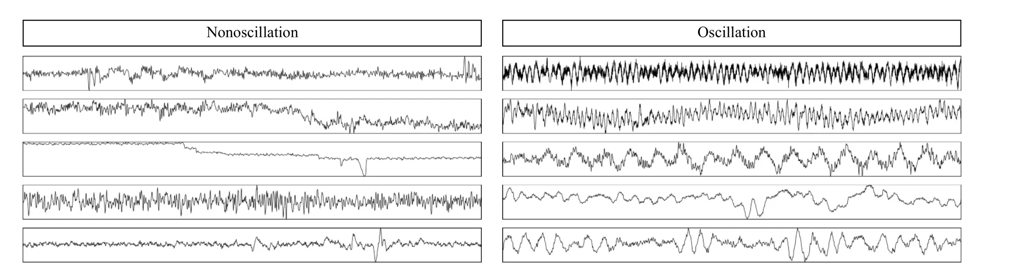
Fig.4.Some simple examples on the industrial dataset.
Furthermore, to ensure that the detection was not influenced by the source of the time series, the magnitude of all time series was normalized to a value equal to 1.
B. Evaluation Metrics
In the field of deep learning, some quantitative metrics are commonly used to evaluate the performance of methods [45].To be inspired, this work proposes to evaluate the effectiveness of the CNNs using the following metrics:
where P and R denote precision and recall, and F1 is a composite measure for P, R.As shown in Table II,TP,TN,FP,andFNdenote the number of true positive, true negative, false positive, and false negative results reported, which are related to the confusion matrix.Since the three metrics above are measures for individual categories, some overall measure is desired in this work.To this end, four metrics, i.e., overall accuracy (OA), average precision (AP), average recall (AR),and average F1 score (AF1) were used, where OA indicates the number of correctly detected samples as a proportion of the total number of samples tested.AP, AR, and AF1 denotethe average of P, R, and F1 indicators for each class, respectively.
TABLE II CONFUSION MATRIX
In addition, detection rate (DR) and average detection time(ADT) were leveraged to check the reliability of the methods.Specifically, DR is defined as the number of samples detected by the techniques used as a percentage of the total number of samples tested.ADT is defined as the average detection time required for each sample tested (including the preprocessing time).
C. Implementation Details
The Keras library was used in this work to build the CNN models with the TensorFlow backend, and Table III lists the corresponding number of learnable parameters (LPs) for each model.With respect to the experimental hyperparameters, an optimal set of hyperparameters enable the best performance of the models.However, the corresponding optimization searchprocess often takes a lot of time, which does not meet the requirements of practical applications.With such consideration, some empirical but widely used hyperparameters were used to train the models.Specifically, the models were trained with an initial learning rate set to 0.001, which was scaled down by a factor of 10 when the loss value was no longer reduced after 16 epochs.The number of epochs was set to 100, and the batch size was set to 4.Moreover, all experiments were repeated five times and then their results were averaged to reduce randomness.Our code was run on a computer with an Intel Pentium G4600 at 3.60 GHz CPU, 8 GB of RAM, and an NVIDIA GeForce GTX 1050 Ti 4GB GPU.
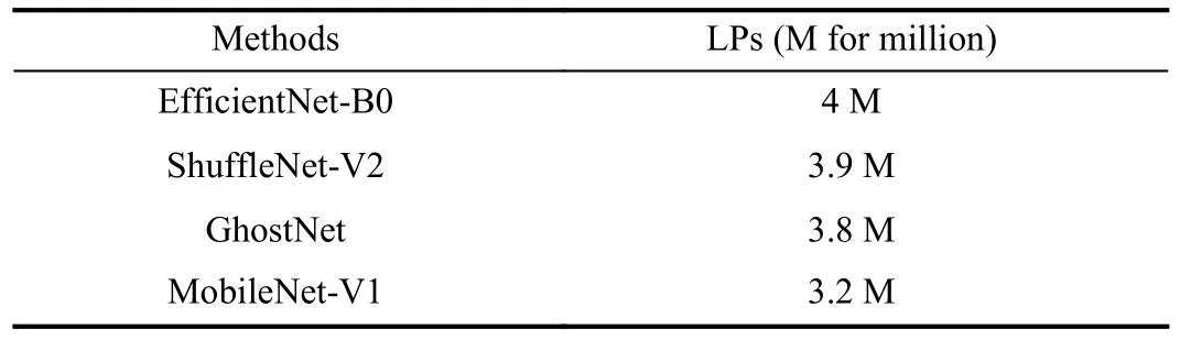
TABLE III NUMBER OF LEARNABLE PARAMETERS
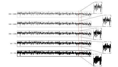
Fig.5.Comparison of sharpness of different resolution images.
D. Performance Evaluation on Artificial Data
A series of numerical experiments were carried out on the artificial data.Firstly, the resolution size used for data imaging was determined experimentally.Secondly, the impact of different data lengths on the performance of visual framework was explored.Thirdly, the lowest signal-to-noise ratio(SNR) allowed for the visual framework to maintain good performance was investigated.Finally, a preliminary evaluation of the detection performance of the four selected CNNs was performed.
1)Ablation Experiments for Resolution: The inherent characteristics of the data are challenging to be detected if the sharpness after imaging is insufficient.To observe the difference, we imaged representative noise data of appropriate length at different resolutions as shown in Fig.5, where the local imaging effect of the noise sequence was amplified.As depicted, the sharpness decreases gradually with decreasing image resolution.In particular, the images with resolutions of 32×384 and 64×768 have only fewer visual features that can be used.Moreover, we also analyzed the difference in detection performance of MobileNet-V1 on different resolution images, as shown in Fig.6.It is observed that the detection performance is positively proportional to the resolution size(here, higher OA and lower loss mean better performance).However, as the resolution gradually increases, the growth trend of the detection performance gradually becomes slower.In view of this, after balancing the accuracy and speed of detection, we set the resolution size of imaging to 200×2400.
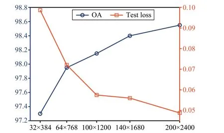
Fig.6.Performance differences of MobileNet-V1 with different resolution images.
2)Ablation Experiments on Data Length: The features of data with different lengths imaged at the same resolution are distinct, which may affect the performance of the visual methods.Given this, we conducted experiments to evaluate the detection performance as a function of the data length.It should be noted foremost that the visual detectability of the oscillation is coupled with its data length and frequency.Therefore, a suitable oscillation frequency needs to be selected before conducting the data length study.To this end,we conducted an extensive review of relevant literature and found that most of the industrial oscillations are repeated at a rate of less than 30 cycles per 1000 sampling points [2], [42],[43].On this basis, we took the highest signal frequency (i.e.,the smallest oscillation period: 1000/30 samples) to explore the performance limits of the visual framework.Specifically,when generating oscillation data of different lengths, the corresponding variables of noise variance (Nvar), disturbance amplitude (Damp) , waveform (Ow f), and smoothing factor(SF) were also set randomly, whose distributions are listed in Table I.In this experiment, the minimum and maximum lengths of the data were set to 200 and 10 000, respectively,based on the observation that most of the industrial oscillations in the relevant industrial datasets are hundreds to thousands of samples long [28], [43].
More specifically, we evaluated the performance of the visual framework at lengths of 200, 1000, 2000, 3000, 4000,5000, 6000, 7000, 8000, 9000, and 10 000, respectively, with the quantitative metric being set to OA.The experimental results are presented in Fig.7, where each listed value is the average of the outcomes of 2000 independent repetitions of the experiment.As illustrated, the performance of all investigated visual methods remains consistently high for most data lengths.However, it is observed that their performance tends to decrease after the data length reaches 8000.We highlight that the above shortcoming has little impact on the practical application of the visual framework given two reasons: a) Due to the slow nature of the industrial processes (low sampling rate), only a few real-world cases have data lengths exceeding 7000; b) The oscillation frequency in this experiment was set to the highest frequency investigated.
3)Ablation Experiments for SNR: The noise resistance of the proposed framework directly affects the effectiveness of detecting industrial oscillations in the presence of noise artifacts.Hence, we would like to explore the lowestSNRallowed for the visual framework to maintain good performance through this experiment.Similar to the experiment of different data lengths, the data used in this experiment were also randomly generated by the generation algorithm of artificial data.The corresponding variables used were signal length(SL) , number of periods (Nper), waveform (Owf), and smoothing factor (S F), whose distributions are listed in Table I.Specifically, we evaluated the performance of the visual framework at differentSNRs of 10, 8, 6, 4, 2, 0, -1, -2, -3,-4, and -5, respectively, with the quantitative metric being set as OA.Here we set the intervals for theSNRs in this way because: whenSNR>0, the performance of four visual methods does not change significantly, so the interval was set to 2.In contrast, whenSNR<0, their changes in performance begin to become progressively significant, so the interval was set to 1.
The experimental results are shown in Fig.8, where each value listed is the average of the outcomes of 2000 independent repetitions of the experiment.From the figure we can make the following observations: a) In the region of highSNR(typicallyS NR≥4), all four visual methods investigated maintain a relatively high level of detection performance; b)In the region of lowSNR(typicallyS NR≤2), the performance of the studied visual methods decreases with decreasingSNR.In particular, afterS NR=0, they will fall below 90% in accuracy; c) For all four visual methods, a significant downward trend can be observed afterS NR=-2, implying thatS NR=-2 may be the beginning of a sharp deterioration in the detection performance of the visual framework.Finally,we would like to note that the lowestSNRthat allows the visual framework to maintain good detection performance is related to a manually set threshold.For example, if the detection accuracy of 90% and below is considered to be unsatisfactory, then the lowestSNRwould be determined to be 2.
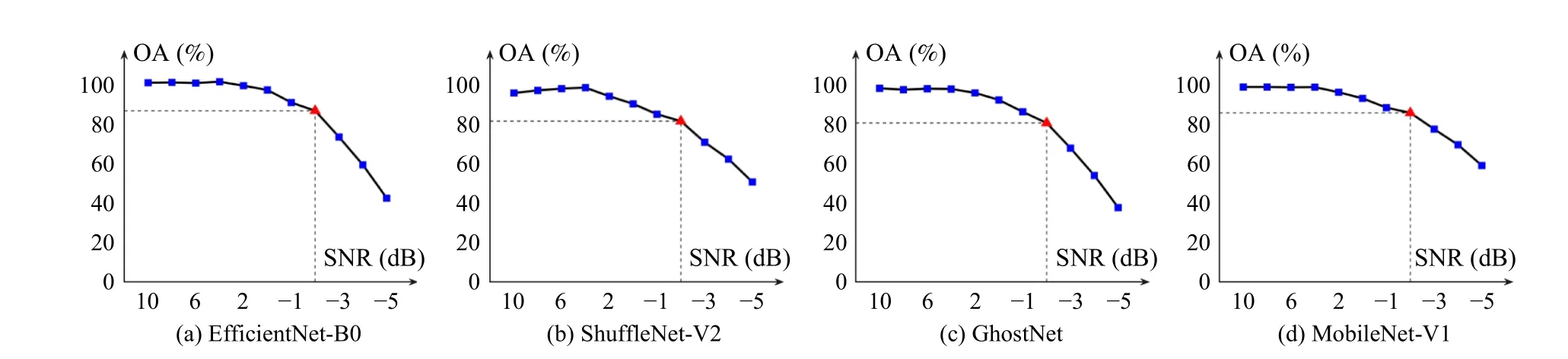
Fig.8.The performance trend of the visual methods at different SNRs.
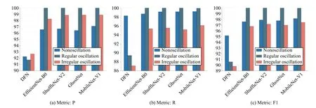
Fig.9.Measure the performance of the models in each class with P, R, and F1 (the closer the numerical result is to 100%, the better).
4)Performance Reported on Artificial Dataset: Here, the deep feedforward network (DFN) proposed by Dambroset al.[28] as an oscillation detector was used for performance comparison to demonstrate the effectiveness of the visual framework using the four selected CNNs.The performance of the methods in each class was measured by three metrics, as shown in Fig.9.As illustrated, the significant difference between the P and R values of DFN in the non-oscillation type reflects the fact that the DFN method is more sensitive to noise and disturbances.When disruptions increase, it directly causes DFN to misclassify the oscillatory time series as the non-oscillation ones.The results associated with F1 in Fig.9(c) consistently support the above analysis.In contrast, the four CNN models we selected show better detection performance for each class, especially for the regular oscillations.Such results verify that the visual methods can better extract features from the data and effectively suppress the counteraction generated by noise and disturbances.
The overall measure is an evaluation of the overall detection ability of the methods.The corresponding results of the four visual methods and DFN are reported in Table IV (where the mean and standard deviation were taken from five experiments).In general, the detection performance of the visual methods is improved by 6 to 7 percentage points over DFN,demonstrating the good generalization capability of the proposed visual framework.
It should be noted that all performance evaluation experiments presented above were conducted using the hold-out method.Therefore, to attenuate the interference brought by the way the dataset is divided, a 5-fold cross-validation experiment was carried out to demonstrate the good generalization of the visual methods.The experiment was conducted on the artificial dataset, whose corresponding results are listed in Table V.As shown, the performance differences between the different visual methods are not significant, but all of them are significantly better than DFN.The results associated with theabove cross-validation experiments are generally consistent with those obtained using the hold-out method.

TABLE IV OVERALL MEASUREMENT REPORT OF THE METHODS ON THE ARTIFICIAL DATASET (HOLD-OUT METHOD)

TABLE V OVERALL MEASUREMENT REPORT OF THE METHODS ON THE ARTIFICIAL DATASET (CROSS-VALIDATION METHOD)
We highlight that relying on artificial data alone does not fully verify the validity of the proposed framework, and therefore, some industrial cases were investigated later for further illustration.
E. Comparison of the Methods on Industrial Data
In addition to DFN, we also implemented several commonly used or state-of-the-art methods for oscillation detec-tion in this comparative experiment.The overall metrics of the performance of the methods are listed in Table VI.As shown,both the ACF ratio and the ACF zero-crossings regularity methods fail to detect oscillations in some cases.This result is expected because these methods are based on specific rules.When no such rules exist in the data, they will fail.The improved local mean decomposition (LMD), fast adaptive chirp mode decomposition (FACMD), and DFN can detect all tested data successfully, however, their AF1 values are relatively inferior, which indicates that fewer samples are correctly detected.Throughout the evaluation results in Table VI,the explored visual methods consistently outperform other methods in terms of detection performance.

TABLE VI OVERALL MEASUREMENT REPORT OF THE METHODS ON THE INDUSTRIAL DATASET
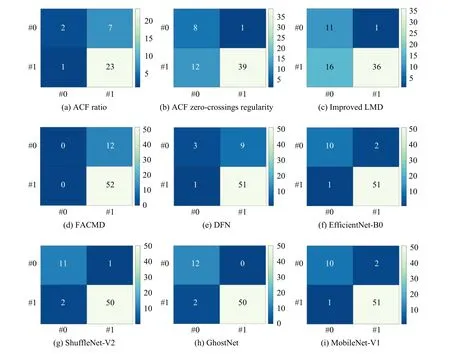
Fig.10.Confusion matrices for each method on the industrial dataset.
It is noteworthy that all comparison methods except the visual ones exhibit significant difference between AP and AR values, which leads to lower AF1 values.To further analyze the cause of this observation, we introduced the confusion matrix.The confusion matrices for all survey methods are shown in Fig.10, from where we observe that the ACF ratio,FACMD, and DFN tend to identify more of the nonoscillation data as oscillatory.In contrast, the ACF zero-crossings regularity and the improved LMD tend to identify more oscillations as nonoscillatory data.The above factors contribute to the lower AP, AR and AF1 values of these methods.In comparison, all visual methods demonstrate high accuracy and strong robustness in detecting oscillations in the presence of noise and mean-nonstationarity.
The speed of detection determines whether the method is reliable in practical applications.Therefore, the detection speed of each method was compared using ADT, and the relevant results are listed in Table VII.As depicted, the detection speed of the improved LMD and the FACMD is significantly slower since they are decomposition-based techniques.Despite the fact that the ACF zero-crossings regularity method has the fastest detection speed, its detection performance (DR)needs to be improved.Furthermore, we highlight that the detection speed of the compared methods is related to the length of the sequence, with longer sequences leading to slower detection speed.In contrast, the visual methods are not influenced by the number of data points.As expected, the visual framework will be quite competitive in terms of detection speed when numerous data points are involved.
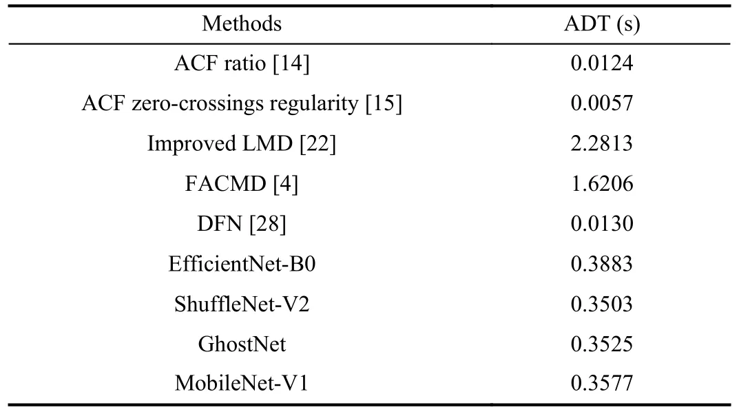
TABLE VII COMPARISON OF THE DETECTION SPEED OF EACH METHOD
V.DISCUSSIONS
Oscillation detection plays a crucial role in monitoring process performance.However, existing methods are poorly generalized and can handle only part of the practical challenges.In view of this, we have explored the feasibility of a visual framework for oscillation detection based on the heuristic definition of oscillation.A set of numerical experiments and industrial cases consistently demonstrated the effectiveness of the proposed framework.
Here, we would like to further discuss the validity of the visual framework in oscillation detection.It should be noted that although oscillation is heuristically defined as periodic abnormal fluctuation visible to the human eye, its detection cannot be regarded as a simple task due to the following reasons: 1) The nature of oscillation varies considerably in terms of length, frequency, and waveform.2) Data collected from process plants are corrupted by noisy artifacts, outliers,unknown disturbances, and nonstationary trends.3) Due to the nonstationary nature of industrial processes, oscillations often suffer from time-varying and intermittent characteristics.4)Multiple oscillatory behaviors caused by multiple fault sources may also coexist.All of the above features seriously degrade the regularity of the oscillation, making its detection a challenging problem [7], [43].Therefore, it can be pointed out that simple machine learning methods have limited representation capability, which makes it difficult for them to effectively capture the oscillatory features of complex industrial processes.This point is also supported by experiments as those shown in Tables IV-VI.Typically, the detection accuracy of DFN, which uses a simple network structure, is significantly worse than that of other visual methods.
In addition, from the industrial dataset, we found that a few samples contain outliers and multiple oscillations, which are not involved in the artificial data in contrast.However, these samples are correctly detected by the visual methods, proving that the proposed framework generalizes well and that we can discover the commonalities of oscillatory time series with different features.To demonstrate more intuitively the verdict ability of the visual framework on oscillation detection, here we embed high-dimensional features into a two-dimensional visualization graph by the uniform manifold approximation and projection (UMAP) algorithm [46].The visualization results of the four selected CNN models on the artificial and industrial datasets are shown in Figs.11 and 12, respectively.It is obvious from Fig.11 that data features extracted by CNNs are well represented and can effectively distinguish among these three types of data.A similar observation can also be drawn in Fig.12.
However, there is still a problem that is demonstrated in Figs.11 and 12 which occurs when the CNN models acquire a sparse distribution of features in each type of data, resulting in poor intra-class compactness.This may be an important cause for their fluctuating detection performance on the industrial dataset (as shown by the standard deviations in Table VI).In response to the above issue, we speculate that there are two possible causes.On the one hand, there may be an inherently large intra-class discrepancy in the training data.However, the main goal of CNN models is not to reduce the intra-class distance, which may lead to poor intra-class compactness of their extracted features.On the other hand, the softmax classifier and loss function are directly related to the sample features mapped in the metric space.Despite their competitive generality, they do not explicitly encourage discriminative learning of features, which results in poor intra-class compactness.Future work will focus on addressing both of the above aspects to better apply visual methods to practical applications in process industries.
VI.CONCLUSION
In this work, we have explored the feasibility of a deep learning-based visual framework for oscillation detection,based on the widely accepted definition of oscillation.Four typical CNNs were applied to this framework separately to evaluate their detection performance.Corresponding representative numerical experiments and industrial cases consistently demonstrated that our proposed framework enables simple and effective oscillation detection for practical applications.However, we highlight that the present work is only a tiny step forward in using visual methods to address the difficulties associated with oscillation monitoring.Many research challenges remain to be solved, such as balancing the image resolution size with the performance of computers when there are too many data points.Furthermore, some more advanced techniques in computer vision, such as metric learning, incremental learning, and transfer learning, have not yet been introduced into this field.In summary, it is encouraged to continue the in-depth research on oscillation detection using visual framework.
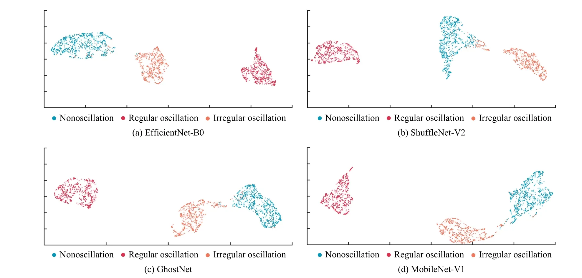
Fig.11.Visualization results on the artificial data.
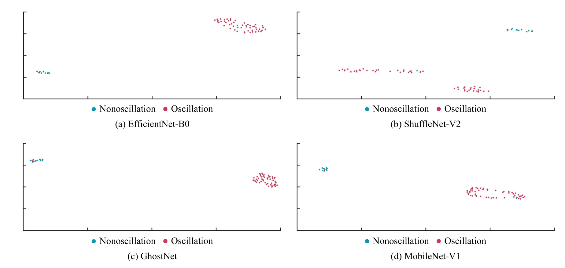
Fig.12.Visualization results on the industrial data.
ACKNOWLEDGMENT
We thank Dambroset al.for making the artificial dataset publicly available.
 IEEE/CAA Journal of Automatica Sinica2024年4期
- IEEE/CAA Journal of Automatica Sinica的其它文章
- When Does Sora Show:The Beginning of TAO to Imaginative Intelligence and Scenarios Engineering
- Goal-Oriented Control Systems (GOCS):From HOW to WHAT
- Digital CEOs in Digital Enterprises: Automating,Augmenting, and Parallel in Metaverse/CPSS/TAOs
- A Tutorial on Federated Learning from Theory to Practice: Foundations, Software Frameworks,Exemplary Use Cases, and Selected Trends
- Cybersecurity Landscape on Remote State Estimation: A Comprehensive Review
- Data-Based Filters for Non-Gaussian Dynamic Systems With Unknown Output Noise Covariance